Introduction to numpy and matplotlib

Note

This material is mostly adapted from the following resources:

• Earth and Environmental Data Science: Numpy and Matplotlib

• Python Programming for Data Science: Chapter 5: Introduction to NumPy

This lecture will introduce NumPy and Matplotlib. Numpy and Matplotlib are two of the most fundamental parts of the scientific python ecosystem. Most of everything else is built on top of them.

Numpy: The fundamental package for scientific computing with Python. NumPy is the standard Python library used for working with arrays (i.e., vectors & matrices), linear algebra, and other numerical computations.

• Website: https://numpy.org/

• GitHub: numpy/numpy

Note

Documentation for this package is available at https://numpy.org/doc/stable/index.html.

Matplotlib: Matplotlib is a comprehensive library for creating static and animated visualizations in Python.

• Website: https://matplotlib.org/

• GitHub: matplotlib/matplotlib

Note

Documentation for this package is available at https://matplotlib.org/stable/index.html.

Note

If you have not yet set up Python on your computer, you can execute this tutorial in your browser via Google Colab. Click on the rocket in the top right corner and launch “Colab”. If that doesn’t work download the .ipynb file and import it in Google Colab

Then install numpy and matplotlib by executing the following command in a Jupyter cell at the top of the notebook.

!pip install matplotlib numpy

Importing Packages

This will be our first experience with importing package.

Usually we import numpy with the alias np. Matplotlib’s plotting module is often imported with the alias plt.

import numpy as np
import matplotlib.pyplot as plt

NDArrays

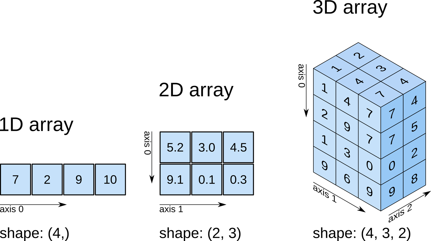
NDarrays (short for n-dimensional arrays) are a key data structure in numpy. NDarrays are similar to Python lists, but they allow for fast, efficient computations on large arrays and matrices of numerical data. NDarrays can have any number of dimensions, and are used for a wide range of numerical and scientific computing tasks.

Thus, the main differences between a numpy array and a list are the following:

• numpy arrays can have N dimensions (while lists only have 1)

• numpy arrays hold values of the same datatype (e.g. int, float), while lists can contain anything.

• numpy optimizes numerical operations on arrays for speed and efficiency.

Numpy arrays can be created in several ways, for example from a Python list:

a = np.array([9, 0, 2, 1, 0])
a

array([9, 0, 2, 1, 0])

b = np.array([[5, 3, 1, 9], [9, 2, 3, 0]], dtype=np.float64)
b

array([[5., 3., 1., 9.],
       [9., 2., 3., 0.]])

Two key properties of numpy arrays are their shape and datatype. The shape of an array describes its dimensions (number of rows and columns), while the datatype describes the type of data stored in the array (e.g., integers, floats, etc.). You can check the shape and datatype of a numpy array using the .shape and .dtype attributes.

a.dtype

dtype('int64')

a.shape

(5,)

b.dtype

dtype('float64')

b.shape

(2, 4)

Creating Arrays

There are many different ways to create arrays, e.g., arrays with all zeros (np.zeros()), all ones (np.ones()), or random values (np.random.rand()), full arrays (np.full()), identity matrices (np.eye()), and more. np.arange() and np.linspace() are useful functions to create arrays with evenly spaced values.

np.zeros((4, 4))

array([[0., 0., 0., 0.],
       [0., 0., 0., 0.],
       [0., 0., 0., 0.],
       [0., 0., 0., 0.]])

np.ones((2, 2, 3))

array([[[1., 1., 1.],
        [1., 1., 1.]],

       [[1., 1., 1.],
        [1., 1., 1.]]])

np.full((3, 2), np.pi)

array([[3.14159265, 3.14159265],
       [3.14159265, 3.14159265],
       [3.14159265, 3.14159265]])

np.random.rand(4, 2)

array([[0.14730608, 0.17176585],
       [0.66036687, 0.1441276 ],
       [0.78736445, 0.1983836 ],
       [0.8964778 , 0.68773584]])

np.arange(10)

array([0, 1, 2, 3, 4, 5, 6, 7, 8, 9])

np.arange(2, 4, 0.25)

array([2.  , 2.25, 2.5 , 2.75, 3.  , 3.25, 3.5 , 3.75])

np.linspace(2, 4, 21)

array([2. , 2.1, 2.2, 2.3, 2.4, 2.5, 2.6, 2.7, 2.8, 2.9, 3. , 3.1, 3.2,
       3.3, 3.4, 3.5, 3.6, 3.7, 3.8, 3.9, 4. ])

Indexing and Slicing

Basic indexing in numpy is similar to lists from standard Python. You can access individual elements of a numpy array using square brackets [] and the index of the element you want to access.

To get a specific element of b, you can use:

b[1, 2]

np.float64(3.0)

To get a specific row of b, you can use:

b[0]

array([5., 3., 1., 9.])

To get a specific column of b, you can use:

# get some whole columns
b[:, 3]

array([9., 0.])

To get a specific range of b, so-called slicing, you can use:

b[0:2, 0:2]

array([[5., 3.],
       [9., 2.]])

Vectorized Operations

Numpy arrays support vectorized operations, which means you can perform operations on entire arrays without the need for explicit loops. This makes computations faster and more efficient. For example, you can add, subtract, multiply, and divide arrays element-wise using standard arithmetic operators. It is particularly useful for mathematical operations on large datasets.

b * 2

array([[10.,  6.,  2., 18.],
       [18.,  4.,  6.,  0.]])

You can also combine arrays element-wise using operations like addition, subtraction, multiplication, and division. For example:

c = np.array([[1, 2, 3, 4], [5, 6, 7, 8]], dtype=np.float64)

b + c

array([[ 6.,  5.,  4., 13.],
       [14.,  8., 10.,  8.]])

There is a range of different mathematical functions available in numpy, such as np.sin(), np.cos(), np.exp(), and more, which can be applied to entire arrays.

np.sin(b)

array([[-0.95892427,  0.14112001,  0.84147098,  0.41211849],
       [ 0.41211849,  0.90929743,  0.14112001,  0.        ]])

To illustrate the power of vectorized operations, consider the following example where we compute the square the the first 100 million integers.

First, with a pure Python loop:

import time
start = time.time()
squares = [x**2 for x in range(100_000_000)]
end = time.time()
print(f"Time taken with pure Python: {end - start:.4f} seconds")

Time taken with pure Python: 5.4658 seconds

Next, using numpy vectorized operations:

start = time.time()
np.arange(100_000_000) ** 2
end = time.time()
print(f"Time taken with NumPy: {end - start:.4f} seconds")

Time taken with NumPy: 0.1952 seconds

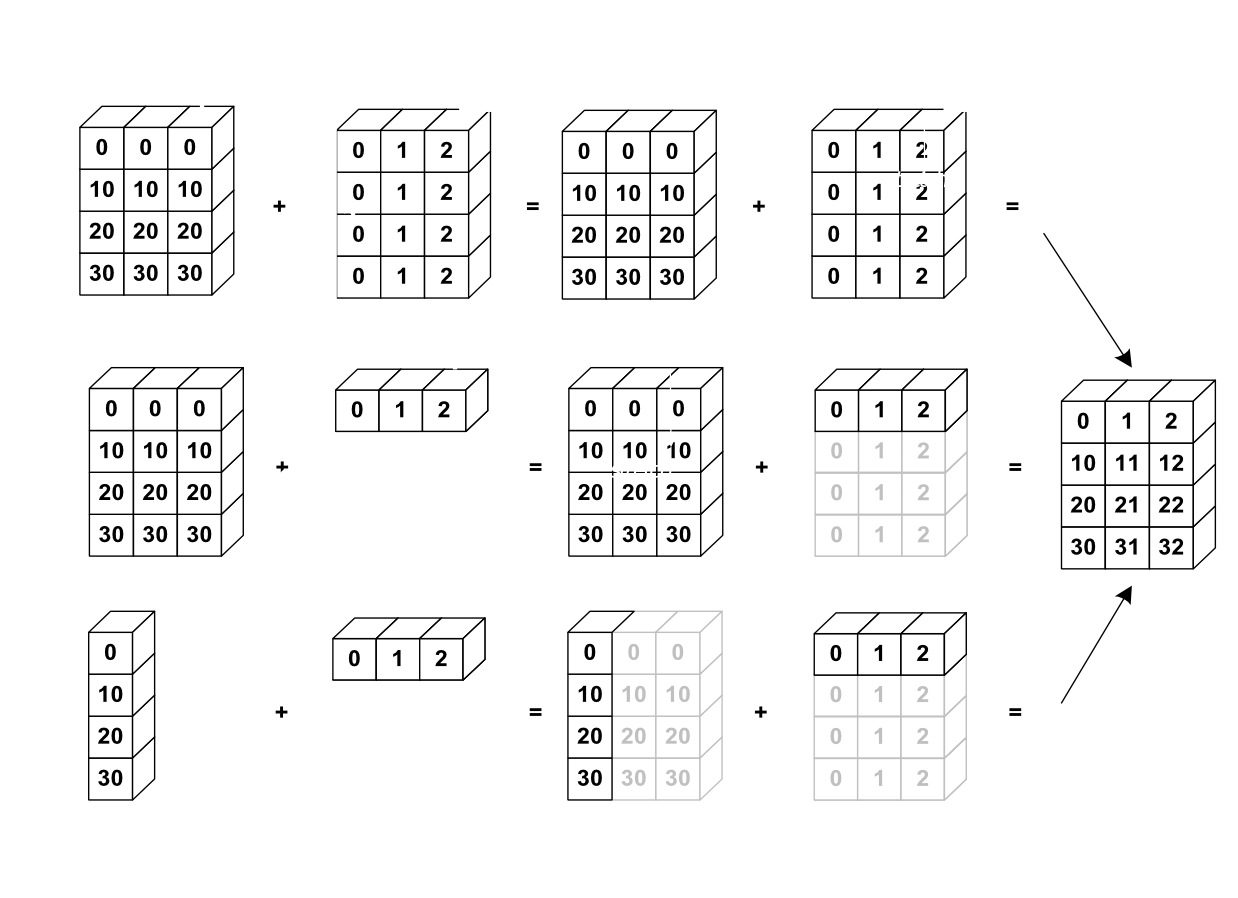
Broadcasting

Not all arrays have to be of the same shape to perform operations together. Numpy uses a powerful mechanism called broadcasting to make arrays with different shapes compatible for arithmetic operations. Broadcasting works by “stretching” the smaller array along the dimensions of the larger array so that they have compatible shapes, without actually copying any data.

d = np.array([10, 20, 30, 40], dtype=np.float64)

b + d

array([[15., 23., 31., 49.],
       [19., 22., 33., 40.]])

Note that broadcasting follows specific rules to determine how arrays can be broadcast together. If one arrays has fewer dimensions, numpy pretends it has extra dimensions of size 1 to the left side (e.g. shape (4,) becomes (1, 4)). The comparison is then made from the right to left (i.e., the last dimension is compared first). Two dimensions are compatible if they are equal, or if one of them is 1. If the dimensions are not compatible, a ValueError is raised.

This example works:

x = np.ones((3, 4))
y = np.array([1, 2, 3, 4])
x + y

array([[2., 3., 4., 5.],
       [2., 3., 4., 5.],
       [2., 3., 4., 5.]])

This example does not work:

x = np.ones((3, 4))
y = np.array([1, 2, 3])
try:
    x + y
except ValueError as e:
    print(e)

operands could not be broadcast together with shapes (3,4) (3,) 

Reduction Operations

Reduction operations are functions that reduce the dimensions of an array by performing a specific operation along a specified axis. Common reduction operations include sum(), mean(), min(), max(), and std() (standard deviation). By specifying the axis parameter, you can control whether the operation is performed across rows (axis=0) or columns (axis=1).

b

array([[5., 3., 1., 9.],
       [9., 2., 3., 0.]])

b.sum()

np.float64(32.0)

b.mean(axis=1)  # mean of each row

array([4.5, 3.5])

b.mean(axis=0)  # mean of each column

array([7. , 2.5, 2. , 4.5])

Boolean Masking

Often, we want to select parts of an array that meet certain conditions. This can be done using boolean masking, where we create a boolean array that indicates which elements of the original array meet the condition, and then use this boolean array to index the original array.

A comparison like >, <, or == produces a boolean array (True/False values) which we can use to filter the data.

values = np.array([10, 20, 30, 40, 50])
mask = values > 25

values[mask]

array([30, 40, 50])

Basic Plotting with Matplotlib

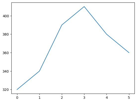
Let’s create some hypothetical electricity demand data for 6 hours:

demand = np.array([320, 340, 390, 410, 380, 360])
hours = np.arange(6)

For plotting such a 1D array as a line, we use the plot function.

plt.plot(hours, demand)

[<matplotlib.lines.Line2D at 0x7fe8a8877350>]

In many cases we would want to adjust the plot, for instance, by adding labels and a title, or by changing the line style or color.

Note

As described in the colors documentation, there are some special codes for commonly used colors. The same applies to line styles and markers (https://matplotlib.org/api/markers_api.html).

plt.plot(hours, demand, marker='o', linestyle='--', color='orange', label='Demand')
plt.xlabel('Hours')
plt.ylabel('Electricity Demand (MW)')
plt.title('Electricity Demand Over 6 Hours')
plt.ylim(0, 500)
plt.legend()
plt.grid()

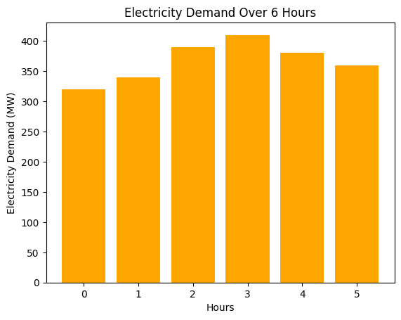
Potentially, we would also like to plot a bar chart instead of a line chart to visualize the electricity demand data.

plt.bar(hours, demand, color='orange', label='Demand')
plt.xlabel('Hours')
plt.ylabel('Electricity Demand (MW)')
plt.title('Electricity Demand Over 6 Hours')

Text(0.5, 1.0, 'Electricity Demand Over 6 Hours')

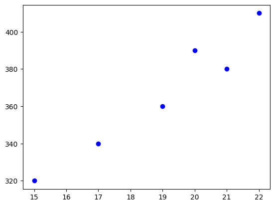
Suppose we want to make a scatter plot between demand data and temperature data. This can be done using the scatter function, which plots the respective data points as individual markers.

temp = np.array([15, 17, 20, 22, 21, 19])
plt.scatter(temp, demand, color='blue')

<matplotlib.collections.PathCollection at 0x7fe7e2c47c50>

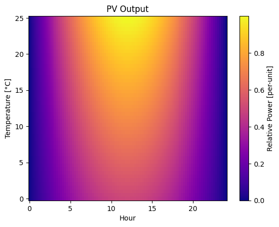
Two-Dimensional Plots

For data depending on two variables, such as hour and temperature, we can use a combination of the meshgrid function to create a grid of coordinates, and the pcolormesh function to create a color-coded 2D plot.

x = np.linspace(0, 24, 100)      # hours
y = np.linspace(0, 25, 50)       # temperatures
xx, yy = np.meshgrid(x, y)

pv_output = np.maximum(0, np.sin(np.pi * xx / 24) * (1 - 0.02 * (25 - yy)))

plt.pcolormesh(xx, yy, pv_output, cmap="plasma")
plt.xlabel("Hour")
plt.ylabel("Temperature [°C]")
plt.title("PV Output")
plt.colorbar(label="Relative Power [per-unit]")

<matplotlib.colorbar.Colorbar at 0x7fe7e2b915d0>

Note

There are many different colormaps available in matplotlib: https://matplotlib.org/stable/tutorials/colors/colormaps.html

Figures and Axes

Every plot created with matplotlib is contained within a figure and one or more axes. Each axis represents a single plot within the figure, and can contain multiple elements such as lines, markers, and labels. Think of it as the canvas (figure) and the individual paintings (axes) on that canvas.

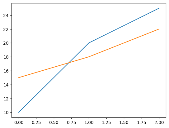
To create a figure with one axis, run:

fig, ax = plt.subplots()
ax.plot([0, 1, 2], [10, 20, 25])
ax.plot([0, 1, 2], [15, 18, 22])

[<matplotlib.lines.Line2D at 0x7fe7e0989cd0>]

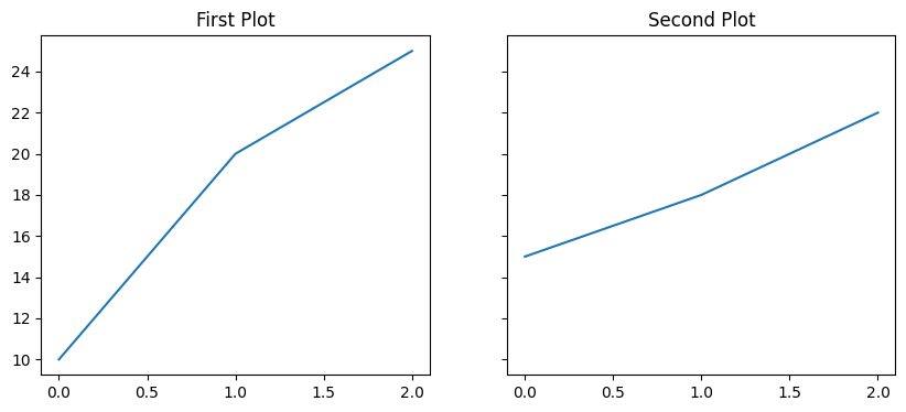
A figure can also contain multiple axes (subplots). This can be useful for comparing multiple plots side by side or in a grid layout. You can create multiple subplots using the subplots function and specifying the number of rows and columns.

fig, axes = plt.subplots(1, 2, figsize=(10, 4), sharey=True)
axes[0].plot([0, 1, 2], [10, 20, 25])
axes[0].set_title('First Plot')
axes[1].plot([0, 1, 2], [15, 18, 22])
axes[1].set_title('Second Plot')

Text(0.5, 1.0, 'Second Plot')

Exercises

1. Create an array with hourly demands 200, 220, 240, 260, 280, and 300 MW. Print its shape and datatype.

2. Create ten evenly spaced temperature values between 15 and 25 degrees Celsius using np.linspace().

3. Print the first 3 values and the last 3 values of the following array:

   demand = np.array([300, 320, 340, 360, 380, 400, 420, 440, 460, 480])
   

4. Convert the following temperature array to a heating energy demand using the formula demand = 1000 - 20 * temperature.

   temperature = np.array([10, 12, 15, 20, 25])
   

5. You have daily demand demand data for 3 days and 3 hours

   demand = np.array([[300, 320, 340],
                      [280, 300, 310],
                      [260, 270, 290]])
   

   Multiply each hour (columns) by scaling factors 0.9, 1.0, and 1.1 respectively using broadcasting. What are the dimensions and values of the resulting array? What do the new values represent?

6. Consider the following values of hourly wind speeds in m/s.

   wind_speeds = np.array([5, 10, 15, 20, 25])
   

   Calculate the average wind speed, minimum wind speed, and maximum wind speed using reduction operations.

7. Consider the following values for demand and generation for 8 hours.

   demand = np.array([400, 420, 450, 480, 500, 520, 550, 580])
   generation = np.array([300, 350, 400, 450, 480, 500, 530, 600])
   

   Create two line plots on the same figure showing both demand and generation over time. Add appropriate labels and a legend.

8. Sometimes we want to compare two different variables side by side. Use subplots to visualize the following demand and price time series over six hours.

   demand = np.array([300, 320, 340, 360, 380, 400])
   price = np.array([50, 55, 60, 65, 70, 75])
   

   Create one figure with two subplots arranged in one row and two columns. The first subplot should show demand over time, and the second subplot should show price over time. Add appropriate titles and labels to each subplot and enable grid lines.