Introduction to geopandas & cartopy

Note

If you have not yet set up Python on your computer, you can execute this tutorial in your browser via Google Colab. Click on the rocket in the top right corner and launch “Colab”. If that doesn’t work download the .ipynb file and import it in Google Colab.

Then install the following packages by executing the following command in a Jupyter cell at the top of the notebook.

!pip install pandas geopandas matplotlib cartopy mapclassify

Why not pandas?

Let’s reload again our example dataset of conventional power plants in Europe as a pd.DataFrame.

import pandas as pd
import matplotlib.pyplot as plt

fn = "https://raw.githubusercontent.com/PyPSA/powerplantmatching/master/powerplants.csv"
ppl = pd.read_csv(fn, index_col=0)

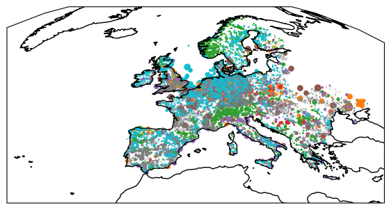
This dataset includes coordinates (latitude and longitude), which allows us to plot the location and capacity of all power plants in a scatter plot:

ppl.plot.scatter("lon", "lat", s=ppl.Capacity / 1e3)

<Axes: xlabel='lon', ylabel='lat'>

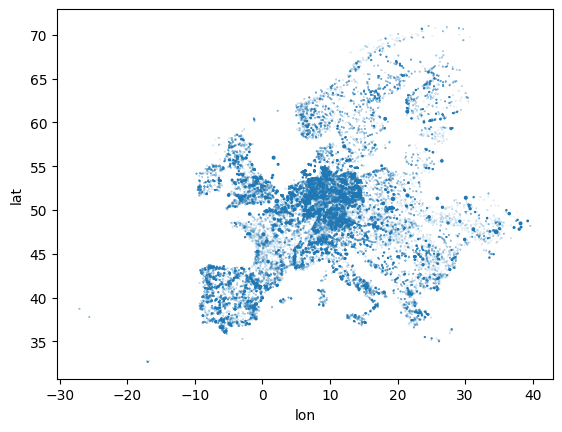
However, this graphs misses some geographic reference point, we’d normally expect for a map like shorelines, country borders and so on.

Why geopandas?

Geopandas extends pandas by adding support for geospatial data.

The core data structure in GeoPandas is the geopandas.GeoDataFrame, a subclass of pandas.DataFrame, that can store geometry columns and perform spatial operations.

Note

Documentation for this package is available at https://geopandas.org/en/stable/.

Typical geometries are points, lines, and polygons. They come from another library called shapely, which helps you create, analyze, and manipulate two-dimensional shapes and their properties, such as points, lines, and polygons.

First, we need to import the geopandas package. The conventional alias is gpd:

import geopandas as gpd

We can convert the latitude and longitude values given in the dataset to formal geometries (to be exact, a shapely.Point object) using the gpd.points_from_xy() function, and use this to gpd.GeoDataFrame. We should also specify a so-called coordinate reference system (CRS). The code 4326 means latitude and longitude values, the so-called WGS84 system.

geometry = gpd.points_from_xy(ppl["lon"], ppl["lat"])
geometry[:5]

<GeometryArray>
[ <POINT (7.324 52.473)>,  <POINT (9.345 53.851)>,  <POINT (3.716 51.433)>,
   <POINT (9.176 49.04)>, <POINT (12.293 48.606)>]
Length: 5, dtype: geometry

gdf = gpd.GeoDataFrame(ppl, geometry=geometry, crs=4326)

Now, the resulting gdf looks like this:

gdf.head(3)

	Name	Fueltype	Technology	Set	Country	Capacity	Efficiency	DateIn	DateRetrofit	DateOut	lat	lon	Duration	Volume_Mm3	DamHeight_m	StorageCapacity_MWh	EIC	projectID	geometry
id
0	Kernkraftwerk Emsland	Nuclear	Steam Turbine	PP	Germany	1336.0	0.33	1988.0	1988.0	2023.0	52.472897	7.32414	NaN	0.0	0.0	0.0	{nan}	{'MASTR': {'MASTR-SEE944567587799'}, 'ENTSOE':...	POINT (7.32414 52.4729)
1	Brokdorf	Nuclear	Steam Turbine	PP	Germany	1410.0	0.33	1986.0	1986.0	2021.0	53.850830	9.34472	NaN	0.0	0.0	0.0	{nan}	{'MASTR': {'MASTR-SEE951462745445'}, 'ENTSOE':...	POINT (9.34472 53.85083)
2	Borssele	Hard Coal	Steam Turbine	PP	Netherlands	485.0	NaN	1973.0	NaN	2034.0	51.433200	3.71600	NaN	0.0	0.0	0.0	{'49W000000000054X'}	{'BEYONDCOAL': {'BEYOND-NL-2'}, 'ENTSOE': {'49...	POINT (3.716 51.4332)

gdf.geometry.head()

id
0     POINT (7.32414 52.4729)
1    POINT (9.34472 53.85083)
2       POINT (3.716 51.4332)
3    POINT (9.17641 49.04002)
4    POINT (12.29315 48.6056)
Name: geometry, dtype: geometry

With the additional geometry columns, it is now even easier to plot the geographic data:

gdf.plot(
    column="Fueltype",
    markersize=gdf.Capacity / 1e2,
)

<Axes: >

We can also start up an interactive map to explore the geodata in more detail:

gdf.explore(column="Fueltype")

Make this Notebook Trusted to load map: File -> Trust Notebook

Projections with cartopy

Cartopy is a Python package designed for geospatial data processing and has an interface for handling projections in matplotlib maps.

Why is it needed?

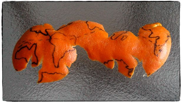
The Earth is a globe, but we present maps usually on two-dimensional surfaces. Hence, we typically need to project data points onto flat surfaces (e.g. screens, paper). However, we will always loose some information in doing so.

A map projection is:

a systematic transformation of the latitudes and longitudes of locations from the surface of a sphere or an ellipsoid into locations on a plane. Wikipedia: Map projection.

Different projections preserve different metric properties. As a result, converting geodata from one projection to another is a common exercise in geographic data science.

• conformal projections preserve angles/directions (e.g. Mercator projection)

• equal-area projections preserve area measure (e.g. Mollweide)

• equidistant projections preserve distances between points (e.g. Plate carrée)

• compromise projections seek to strike a balance between distortions (e.g. Robinson)

If you like the “Orange-as-Earth” analogy for projections, checkout this numberphile video by Hannah Fry.

Note

Documentation for this package is available at https://scitools.org.uk/cartopy/docs/latest/.

First, we need to import the relevant parts of the cartopy package:

import cartopy
import cartopy.crs as ccrs

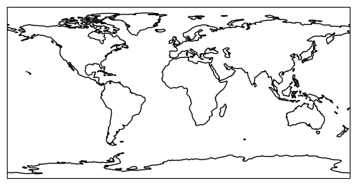
Let’s draw a first map with cartopy outlining the global coastlines in the so-called plate carrée projection (equirectangular projection):

ax = plt.axes(projection=ccrs.PlateCarree())
ax.coastlines()

<cartopy.mpl.feature_artist.FeatureArtist at 0x7fb3886723c0>

Note

A list of the available projections can be found on the Cartopy projection list page.

We can combine the functionality of cartopy with geopandas plots and even add geographical features:

fig = plt.figure(figsize=(7, 7))

ax = plt.axes(projection=ccrs.PlateCarree())

gdf.plot(
    ax=ax,
    column="Fueltype",
    markersize=gdf.Capacity / 1e2,
)

ax.coastlines()

ax.add_feature(cartopy.feature.BORDERS, color="red", linewidth=0.5)

ax.add_feature(cartopy.feature.OCEAN, color="blue")

ax.add_feature(cartopy.feature.LAND, color="yellow");

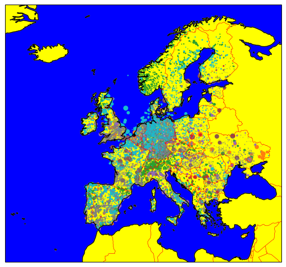
Geopandas will automatically calculate sensible bounds for the plot given the geographic data. But we can also manually zoom in or out by setting the spatial extent with the .set_extent() method:

ax.set_extent([5, 16, 47, 55])
fig

Reprojecting a GeoDataFrame

In geopandas, we can use the function .to_crs() to convert a GeoDataFrame with a given projection to another desired target coordinate reference system, using a cartopy CRS object:

crs = ccrs.Orthographic()
print(crs)

+proj=ortho +a=6378137.0 +lon_0=0.0 +lat_0=0.0 +alpha=0.0 +no_defs +type=crs

gdf.to_crs(crs).geometry.head()

id
0    POINT (495289.543 5058279.038)
1    POINT (610915.426 5150243.264)
2    POINT (257707.919 4986949.543)
3    POINT (666775.128 4816562.597)
4    POINT (897956.621 4784723.399)
Name: geometry, dtype: geometry

fig = plt.figure(figsize=(7, 7))

ax = plt.axes(projection=crs)

gdf.to_crs(crs).plot(
    ax=ax,
    column="Fueltype",
    markersize=gdf.Capacity / 1e2,
)

ax.coastlines()

<cartopy.mpl.feature_artist.FeatureArtist at 0x7fb386bc4a50>

Reading and Writing Files

In the following example, we’ll load a dataset containing the NUTS regions:

Nomenclature of Territorial Units for Statistics or NUTS (French: Nomenclature des unités territoriales statistiques) is a geocode standard for referencing the subdivisions of countries for statistical purposes.

Our ultimate goal for this part of the tutorial is to map the power plant capacities to the NUTS-1 region they belong to.

Common filetypes for vector-based geospatial datasets are GeoPackage (.gpkg), GeoJSON (.geojson), File Geodatabase (.gdb), or Shapefiles (.shp).

In geopandas we can use the gpd.read_file() function to read such files. So let’s start:

url = "https://tubcloud.tu-berlin.de/s/RHZJrN8Dnfn26nr/download/NUTS_RG_10M_2021_4326.geojson"

nuts = gpd.read_file(url)

nuts.head(3)

	id	NUTS_ID	LEVL_CODE	CNTR_CODE	NAME_LATN	NUTS_NAME	MOUNT_TYPE	URBN_TYPE	COAST_TYPE	FID	geometry
0	BG423	BG423	3	BG	Pazardzhik	Пазарджик	3.0	2	3	BG423	POLYGON ((24.42101 42.55306, 24.41032 42.4695,...
1	BG424	BG424	3	BG	Smolyan	Смолян	3.0	3	3	BG424	POLYGON ((25.07422 41.79348, 25.05851 41.75177...
2	BG425	BG425	3	BG	Kardzhali	Кърджали	3.0	3	3	BG425	POLYGON ((25.94863 41.32034, 25.90644 41.30757...

It is good practice to set an index. You can use .set_index() for that:

nuts = nuts.set_index("id")

We can also check out the geometries in the dataset with .geometry:

nuts.geometry

id
BG423    POLYGON ((24.42101 42.55306, 24.41032 42.4695,...
BG424    POLYGON ((25.07422 41.79348, 25.05851 41.75177...
BG425    POLYGON ((25.94863 41.32034, 25.90644 41.30757...
CH011    MULTIPOLYGON (((6.86623 46.90929, 6.89621 46.9...
CH012    POLYGON ((8.47767 46.5276, 8.39953 46.48872, 8...
                               ...                        
LV       POLYGON ((27.35158 57.51824, 27.54521 57.53444...
ME       POLYGON ((20.06394 43.00682, 20.32958 42.91149...
MK       POLYGON ((22.36021 42.31116, 22.51041 42.15516...
SK0      POLYGON ((19.88393 49.20418, 19.96275 49.23031...
IT       MULTIPOLYGON (((12.47792 46.67984, 12.69064 46...
Name: geometry, Length: 2010, dtype: geometry

With .crs we can check in which coordinate reference system the data is given:

nuts.crs

<Geographic 2D CRS: EPSG:4326>
Name: WGS 84
Axis Info [ellipsoidal]:
- Lat[north]: Geodetic latitude (degree)
- Lon[east]: Geodetic longitude (degree)
Area of Use:
- name: World.
- bounds: (-180.0, -90.0, 180.0, 90.0)
Datum: World Geodetic System 1984 ensemble
- Ellipsoid: WGS 84
- Prime Meridian: Greenwich

With .total_bounds we can check the bounding box of the data in the original coordinate reference system:

nuts.total_bounds

array([-63.08825, -21.38917,  55.83616,  80.76427])

Let’s now filter the GeoDataFrame by NUTS-1 level…

nuts1 = nuts.query("LEVL_CODE == 1")

… and explore what kind of geometries we have in the dataset …

nuts1.explore()

Make this Notebook Trusted to load map: File -> Trust Notebook

Note

In principle, the geopandas.GeoDataFrame behaves like a normal pandas.DataFrame and we can use all the familiar pandas functionality plus the geospatial extensions.

To write a GeoDataFrame back to file use GeoDataFrame.to_file(). The file format is inferred from the file ending.

nuts1.to_file("tmp.geojson")

Buffers and Areas

Many geospatial analyses require the calculation of areas or buffers around geometries. However, these calculations depend on the coordinate reference system used.

The first thing we need to do in order to calculate area or buffers is to reproject the GeoDataFrame to an equal-area projection (here: EPSG:3035 which is valid only within Europe; a globally valid alternative is the Mollweide projection EPSG:54009)

nuts1 = nuts1.to_crs(3035)

The area can be accessed via .area and is given in m² (after projection). Let’s convert to km²:

area = nuts1.area / 1e6
area.head()

id
AT1    23545.286205
AT2    25894.953057
EL4    17388.679384
EE0    45315.713593
EL3     3799.676547
dtype: float64

nuts1.explore(column=area, vmax=1e5)

Make this Notebook Trusted to load map: File -> Trust Notebook

We can also build a buffer of 1km around each geometry using .buffer():

nuts1.buffer(1000).explore()

Make this Notebook Trusted to load map: File -> Trust Notebook

It is also possible to calculate the centroid of each geometry, which is the geometric center of a shape. It can be useful for labelling or constructing a point-based network representation of polygonal data:

ax = nuts1.geometry.plot()
nuts1.representative_point().plot(ax=ax, color="red", markersize=2)

<Axes: >

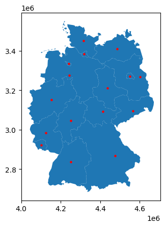
To calculate the distance between two points (or geometries more generally), we can use the .distance() method. For instance, using the nuts1.representative_point() method, we can find a central point that represents each geometry but other than the centroid is guaranteed to be within the geometry. However, note that the distance is only meaningful if the geometries are in an appropriate projected coordinate reference system (e.g. an equidistant projection):

nuts1_de = nuts1.query("CNTR_CODE == 'DE'")
points = nuts1_de.representative_point()

ax = nuts1_de.plot()
points.plot(ax=ax, color="red", markersize=5)

<Axes: >

distances = (
    pd.concat({k: points.distance(p) for k, p in points.items()}, axis=1)
    .div(1e3)
    .astype(int)
)  # km
distances

	DEF	DEG	DE8	DE9	DEA	DEB	DEC	DED	DEE	DE1	DE2	DE3	DE4	DE5	DE6	DE7
id
DEF	0	371	175	189	340	502	569	434	268	616	604	295	340	136	67	408
DEG	371	0	326	250	267	305	354	152	121	301	232	227	258	297	305	167
DE8	175	326	0	278	422	557	620	324	204	618	541	152	183	256	170	432
DE9	189	250	278	0	153	313	379	370	204	438	469	309	359	59	131	229
DEA	340	267	422	153	0	168	233	417	290	329	429	417	464	204	285	144
DEB	502	305	557	313	168	0	66	453	384	194	368	513	553	369	442	140
DEC	569	354	620	379	233	66	0	495	442	174	378	570	608	435	508	195
DED	434	152	324	370	417	453	495	0	173	405	244	177	176	403	379	317
DEE	268	121	204	204	290	384	442	173	0	417	345	130	175	230	208	247
DE1	616	301	618	438	329	194	174	405	417	0	225	528	554	498	550	209
DE2	604	232	541	469	429	368	378	244	345	225	0	411	418	522	538	286
DE3	295	227	152	309	417	513	570	177	130	528	411	0	50	316	258	375
DE4	340	258	183	359	464	553	608	176	175	554	418	50	0	366	306	414
DE5	136	297	256	59	204	369	435	403	230	498	522	316	366	0	90	288
DE6	67	305	170	131	285	442	508	379	208	550	538	258	306	90	0	343
DE7	408	167	432	229	144	140	195	317	247	209	286	375	414	288	343	0

The .distance() function uses the haversine formula to calculate the great-circle distance between two points on the Earth’s surface, given their latitude and longitude coordinates.

Note

See also https://en.wikipedia.org/wiki/Haversine_formula

Dissolve

The .dissolve() function is used to aggregate geometries within a GeoDataFrame based on a specified attribute or set of attributes. Practically, it is very similar to the pandas.DataFrame.groupby() function, but instead of aggregating numerical values, it merges geometries.

For instance, we can dissolve the NUTS regions by country code to get country-level geometries:

nuts1.dissolve("CNTR_CODE")  # .plot()

	geometry	NUTS_ID	LEVL_CODE	NAME_LATN	NUTS_NAME	MOUNT_TYPE	URBN_TYPE	COAST_TYPE	FID
CNTR_CODE
AL	POLYGON ((5129209.756 2204391.664, 5130223.807...	AL0	1	Shqipëria	Shqipëria	0.0	0	0	AL0
AT	POLYGON ((4780562.18 2637267.022, 4763403.161 ...	AT1	1	Ostösterreich	Ostösterreich	0.0	0	0	AT1
BE	POLYGON ((4046990.566 3074015.927, 4051165.103...	BE1	1	Région de Bruxelles-Capitale/Brussels Hoofdste...	Région de Bruxelles-Capitale/Brussels Hoofdste...	0.0	0	0	BE1
BG	POLYGON ((5689130.877 2238900.025, 5687390.983...	BG3	1	Severna i Yugoiztochna Bulgaria	Северна и Югоизточна България	0.0	0	0	BG3
CH	POLYGON ((4221123.396 2731035.643, 4230515.051...	CH0	1	Schweiz/Suisse/Svizzera	Schweiz/Suisse/Svizzera	0.0	0	0	CH0
CY	POLYGON ((6342716.316 1629585.624, 6343492.856...	CY0	1	Kýpros	Κύπρος	0.0	0	0	CY0
CZ	POLYGON ((4623549.852 3113763.529, 4630550.464...	CZ0	1	Česko	Česko	0.0	0	0	CZ0
DE	MULTIPOLYGON (((4104078.126 2901809.263, 40921...	DEF	1	Schleswig-Holstein	Schleswig-Holstein	0.0	0	0	DEF
DK	MULTIPOLYGON (((4352570.618 3531502.278, 43539...	DK0	1	Danmark	Danmark	0.0	0	0	DK0
EE	MULTIPOLYGON (((5053321.816 3962248.087, 50563...	EE0	1	Eesti	Eesti	0.0	0	0	EE0
EL	MULTIPOLYGON (((5490401.282 1553676.16, 548671...	EL4	1	Nisia Aigaiou, Kriti	Νησιά Αιγαίου, Κρήτη	0.0	0	0	EL4
ES	MULTIPOLYGON (((1816703.253 962897.033, 181355...	ES1	1	Noroeste	Noroeste	0.0	0	0	ES1
FI	MULTIPOLYGON (((4878203.934 4138951.764, 48779...	FI2	1	Åland	Åland	0.0	0	0	FI2
FR	MULTIPOLYGON (((-2485479.019 727894.26, -24892...	FRY	1	RUP FR — Régions Ultrapériphériques Françaises	RUP FR — Régions Ultrapériphériques Françaises	0.0	0	0	FRY
HR	MULTIPOLYGON (((4725678.893 2334407.525, 47186...	HR0	1	Hrvatska	Hrvatska	0.0	0	0	HR0
HU	POLYGON ((4912119.551 2767793.968, 4967369.068...	HU1	1	Közép-Magyarország	Közép-Magyarország	0.0	0	0	HU1
IE	MULTIPOLYGON (((2946631.143 3360657.795, 29486...	IE0	1	Ireland	Ireland	0.0	0	0	IE0
IS	MULTIPOLYGON (((2856046.516 4805353.836, 28569...	IS0	1	Ísland	Ísland	0.0	0	0	IS0
IT	MULTIPOLYGON (((4502128.921 1530792.048, 45056...	ITG	1	Isole	Isole	0.0	0	0	ITG
LI	POLYGON ((4292201.608 2670972.476, 4291125.192...	LI0	1	Liechtenstein	Liechtenstein	0.0	0	0	LI0
LT	POLYGON ((5298223.347 3769132.733, 5302391.374...	LT0	1	Lietuva	Lietuva	0.0	0	0	LT0
LU	POLYGON ((4044953.68 3009232.416, 4043779.234 ...	LU0	1	Luxembourg	Luxembourg	0.0	0	0	LU0
LV	POLYGON ((5350178.114 3949791.201, 5360936.766...	LV0	1	Latvija	Latvija	0.0	0	0	LV0
ME	POLYGON ((5141136.882 2266080.654, 5163988.264...	ME0	1	Crna Gora	Црна Гора	0.0	0	0	ME0
MK	POLYGON ((5338319.874 2217739.771, 5353216.719...	MK0	1	Severna Makedonija	Северна Македонија	0.0	0	0	MK0
MT	MULTIPOLYGON (((4716439.646 1441567.871, 47152...	MT0	1	Malta	Malta	0.0	0	0	MT0
NL	MULTIPOLYGON (((4051440.947 3178950.962, 40513...	NL1	1	Noord-Nederland	Noord-Nederland	0.0	0	0	NL1
NO	MULTIPOLYGON (((4056290.045 4007001.29, 405813...	NO0	1	Norge	Norge	0.0	0	0	NO0
PL	MULTIPOLYGON (((5130043.711 2983158.146, 51211...	PL2	1	Makroregion południowy	Makroregion południowy	0.0	0	0	PL2
PT	MULTIPOLYGON (((1223162.364 2516975.095, 12214...	PT1	1	Continente	Continente	0.0	0	0	PT1
RO	POLYGON ((5664979.109 2489203.673, 5654081.733...	RO1	1	Macroregiunea Unu	Macroregiunea Unu	0.0	0	0	RO1
RS	POLYGON ((5221479.991 2476681.501, 5235511.756...	RS1	1	Serbia - sever	Србија - север	0.0	0	0	RS1
SE	MULTIPOLYGON (((4489805.027 3645262.593, 44877...	SE3	1	Norra Sverige	Norra Sverige	0.0	0	0	SE3
SI	POLYGON ((4827386.296 2618351.084, 4810186.907...	SI0	1	Slovenija	Slovenija	0.0	0	0	SI0
SK	POLYGON ((5038951.091 2947340.783, 5044250.649...	SK0	1	Slovensko	Slovensko	0.0	0	0	SK0
TR	MULTIPOLYGON (((5747102.575 1857139.853, 57442...	TR6	1	Akdeniz	Akdeniz	0.0	0	0	TR6
UK	MULTIPOLYGON (((3165171.851 3112814.849, 31622...	UKK	1	South West (England)	South West (England)	0.0	0	0	UKK

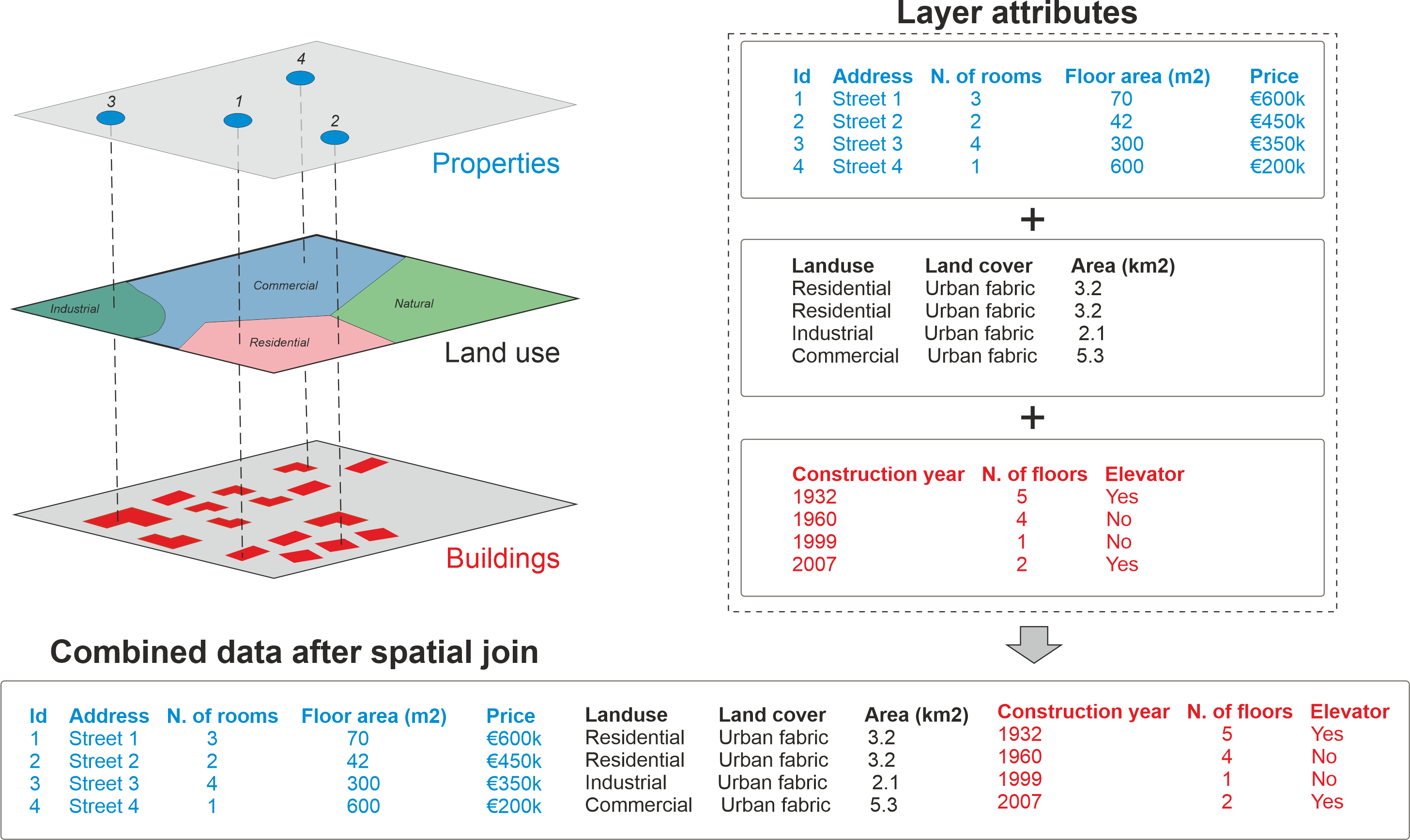
Spatial Joins

Multiple GeoDataFrames can be combined via spatial joins.

Observations from two datasets are combined with the .sjoin() function based on their spatial relationship to one another (e.g. whether they are intersecting, overlapping or contained within one another). You can read more about the specific options here.

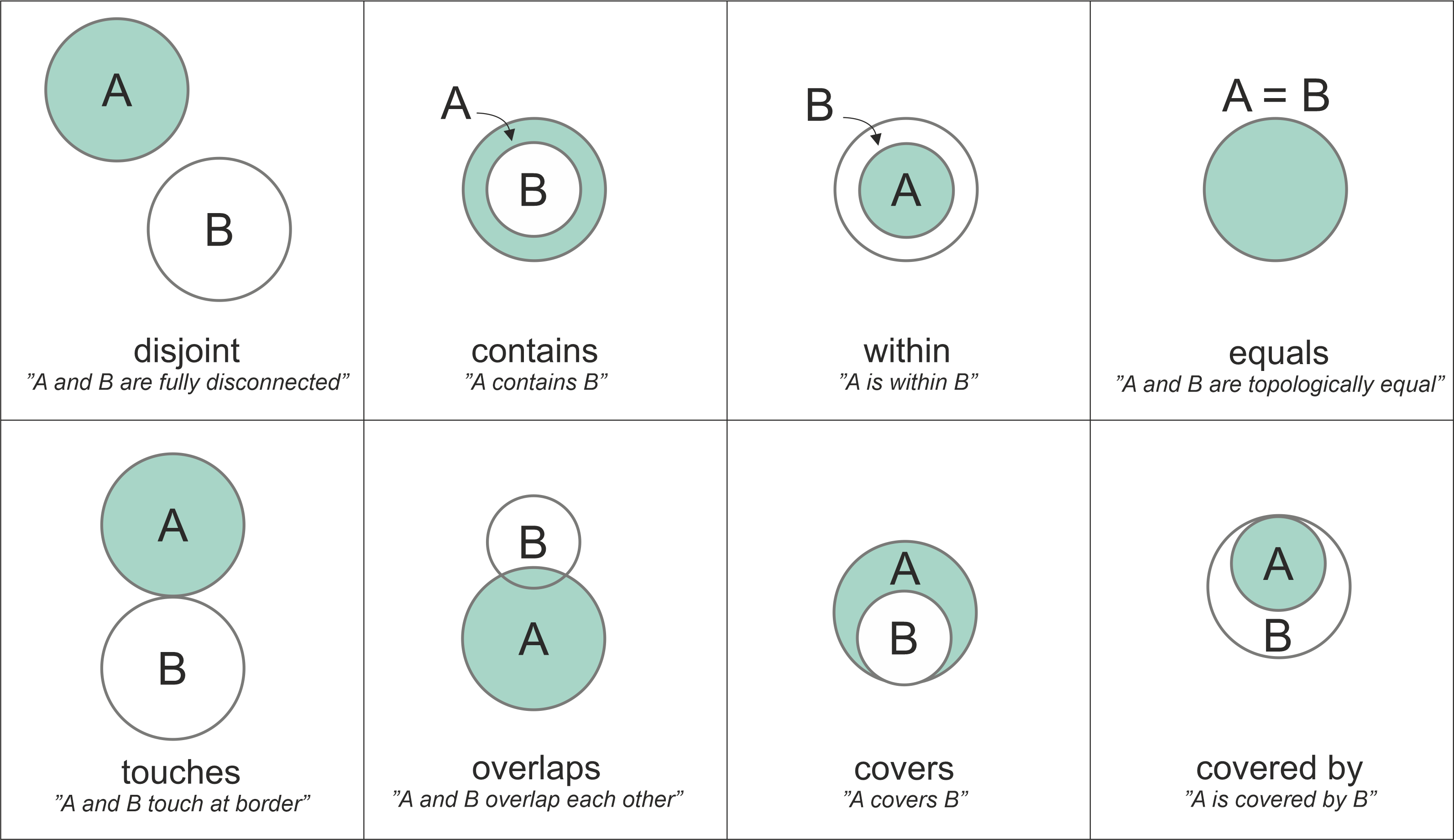
Source: https://pythongis.org

To perform a spatial join, you need to provide the following information:

• The two geopandas.GeoDataFrame objects you want to join (e.g., left_df and right_df).

• The type of spatial relationship to test (e.g., intersects, contains, within). This is specified using the predicate parameter.

• The type of join to perform (e.g., inner, left, right). This is specified using the how parameter. When using left, the resulting GeoDataFrame will retain all records from the left_df, while matching records from the right_df will be added where the spatial relationship holds true. With inner, only records with matches in both GeoDataFrames will be retained. With right, all records from the right_df will be retained, with matching records from the left_df added where applicable.

The .sjoin() function will then go through the geometries in both GeoDataFrames, evaluate the specified spatial relationship, and join the matching records (behind the scenes, it uses spatial indexing to speed up the process).

For example, if the predicate parameter is set to 'intersects', the function will check if the geometries of each record in left_df intersect with the geometries of any records in right_df. If a match is found, the attributes of the corresponding records from both GeoDataFrames will be combined into a new record in the output GeoDataFrame.

Source: https://pythongis.org

The result of the spatial join is a new GeoDataFrame that retains the geometries from the left_df and includes attributes from both GeoDataFrames for the matching records.

When no match is found, the resulting attributes from the right_df will be set to NaN (e.g. when some power plants are located outside of NUTS-1 regions).

Let’s do an example, starting with first reprojecting the gdf object of power plant to the same CRS as nuts1 polygons and reducing it to coal plants:

gdf = gdf.to_crs(3035).query("Fueltype == 'Nuclear'")

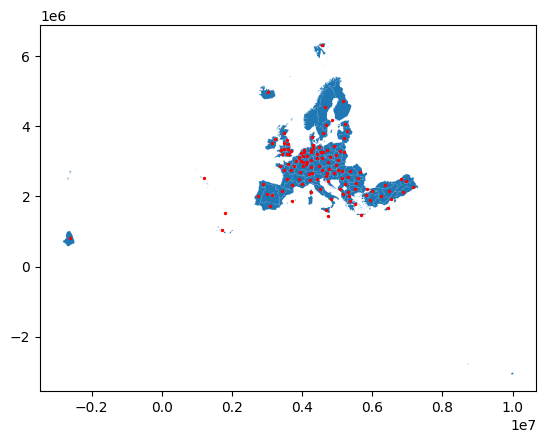
Then, let’s have a look at both datasets at once. We want to find out which points (i.e. the power plants) lie within which shape (i.e. the NUTS1 regions).

fig = plt.figure(figsize=(7, 7))

ax = plt.axes(projection=ccrs.epsg(3035))

nuts1.plot(ax=ax, edgecolor="black", facecolor="sandybrown")

gdf.to_crs(3035).plot(
    ax=ax, column="Fueltype", markersize=gdf.Capacity / 40, legend=True
)

ax.set_extent([-7, 24, 40, 62])

We can now apply the .sjoin() function. By default, .sjoin() looks for intersections and keeps the geometries of the left GeoDataFrame.

joined = gdf.sjoin(nuts1)

If we look at this new GeoDataFrame, we now have additional columns from the NUTS1 data:

joined.head(3)

	Name	Fueltype	Technology	Set	Country	Capacity	Efficiency	DateIn	DateRetrofit	DateOut	...	id_right	NUTS_ID	LEVL_CODE	CNTR_CODE	NAME_LATN	NUTS_NAME	MOUNT_TYPE	URBN_TYPE	COAST_TYPE	FID
id_left
0	Kernkraftwerk Emsland	Nuclear	Steam Turbine	PP	Germany	1336.0	0.33	1988.0	1988.0	2023.0	...	DE9	DE9	1	DE	Niedersachsen	Niedersachsen	0.0	0	0	DE9
1	Brokdorf	Nuclear	Steam Turbine	PP	Germany	1410.0	0.33	1986.0	1986.0	2021.0	...	DEF	DEF	1	DE	Schleswig-Holstein	Schleswig-Holstein	0.0	0	0	DEF
3	Gemeinschaftskernkraftwerk Neckarwestheim	Nuclear	Steam Turbine	PP	Germany	1310.0	0.33	1976.0	1989.0	2023.0	...	DE1	DE1	1	DE	Baden-Württemberg	Baden-Württemberg	0.0	0	0	DE1

3 rows × 29 columns

We can now use these new columns for .groupby() operations on the capacities (as well as sorting, converting values to a suitable unit and renaming the index from NUTS identifiers to NUTS region names):

cap = joined.groupby("NUTS_ID").Capacity.sum().sort_values(ascending=False) / 1000  # GW
cap.rename(nuts1.NUTS_NAME).head(3)

NUTS_ID
Auvergne-Rhône-Alpes     14.812
Grand Est                12.580
Centre — Val de Loire    11.630
Name: Capacity, dtype: float64

With our intersection and left join, some NUTS1 regions disappear in cap because they do not have any power plants. We can fix this by reindexing cap to the full set of NUTS1 regions:

nuts1.index.difference(cap.index)

Index(['AL0', 'AT1', 'AT2', 'AT3', 'BE1', 'BG4', 'CY0', 'DE3', 'DE5', 'DE6',
       'DE8', 'DEC', 'DED', 'DEE', 'DEG', 'DK0', 'EE0', 'EL3', 'EL4', 'EL5',
       'EL6', 'ES1', 'ES2', 'ES3', 'ES6', 'ES7', 'FI1', 'FI2', 'FR1', 'FRC',
       'FRG', 'FRL', 'FRM', 'FRY', 'HR0', 'HU1', 'HU3', 'IE0', 'IS0', 'ITG',
       'LI0', 'LU0', 'LV0', 'ME0', 'MK0', 'MT0', 'NL1', 'NL3', 'NL4', 'NO0',
       'PL2', 'PL4', 'PL5', 'PL6', 'PL7', 'PL8', 'PL9', 'PT1', 'PT2', 'PT3',
       'RO1', 'RO3', 'RO4', 'RS1', 'RS2', 'SE2', 'SE3', 'TR1', 'TR2', 'TR3',
       'TR4', 'TR5', 'TR6', 'TR7', 'TR8', 'TR9', 'TRA', 'TRB', 'TRC', 'UKE',
       'UKF', 'UKG', 'UKI', 'UKJ', 'UKN'],
      dtype='object')

cap = cap.reindex(nuts1.index)
cap.head(3)

id
AT1   NaN
AT2   NaN
EL4   NaN
Name: Capacity, dtype: float64

Additionally, some power plants might be located outside of NUTS1 regions (e.g. the ones in Ukraine). Hence, the total capacity in cap is lower than the total capacity in gdf.

cap.sum() < gdf.Capacity.div(1e3).sum()

np.True_

Finally, we can plot the total hard coal generation capacity per NUTS1 region on a map. For regions without any coal power plants we can use the missing_kwds parameter to set a specific appearance (here red hatching).

fig = plt.figure(figsize=(7, 7))

ax = plt.axes(projection=ccrs.epsg(3035))

nuts1.plot(
    ax=ax,
    column=cap,
    legend=True,
    missing_kwds={
        "color": "lightgrey",
        "edgecolor": "red",
        "hatch": "///",
    },
    legend_kwds={"label": "Hard Coal Capacity [GW]", "shrink": 0.7},
)

ax.set_extent([-7, 24, 40, 62])

This concludes the geopandas and cartopy tutorial!

Note

The key aspect to remember is that aligning coordinate reference systems / projections is crucial when combining data from different geospatial datasets.

Exercises

Take the following code snippet as a starting point. It loads the NUTS regions of Europe, the power plant dataset, and a shapefile for the Danish Natura2000 natural protection areas.

import cartopy
import pandas as pd
import geopandas as gpd
import cartopy.crs as ccrs
import matplotlib.pyplot as plt

url = "https://tubcloud.tu-berlin.de/s/RHZJrN8Dnfn26nr/download/NUTS_RG_10M_2021_4326.geojson"
nuts = gpd.read_file(url)

fn = "https://raw.githubusercontent.com/PyPSA/powerplantmatching/master/powerplants.csv"
df = pd.read_csv(fn, index_col=0)
geometry = gpd.points_from_xy(df["lon"], df["lat"])
ppl = gpd.GeoDataFrame(df, geometry=geometry, crs=4326)

url = "https://tubcloud.tu-berlin.de/s/mEpdmgBtmMbyjAr/download/Natura2000_end2021-DK.gpkg"
natura = gpd.read_file(url)

Task 1: Identify the coordinate reference system of the natura GeoDataFrame.

Task 2: Plot the natura GeoDataFrame on a map without transforming its CRS. Use cartopy for setting the projection of the figure and add coastlines and borders.

Task 3: Identify the name of the largest protected area in the natura GeoDataFrame.

Task 4: What is the total protection area in square kilometers.

Task 5: The natura GeoDataFrame has a column SITETYPE that indicates the type of protected area. Calculate the total area for each type of protected area (again in square kilometers).

Task 6: By how much (in percent) would the total area of protected areas increase if a buffer of 1 km around each protected area were also protected?

Task 7: List the power plants that are located within protected areas. How many power plants are located within protected areas? Use the .sjoin() function. Check the result by plotting these power plants on top of the protected areas.

Task 8 (advanced): What fraction of the natural protection area is located offshore? Use set operations with the .overlay() function and the NUTS regions GeoDataFrame.

Note

Consult the GeoPandas documentation if you need an introduction to how to use the .overlay() function.