Solution pandas#
Power Plants Data#
In this exercise, we will use the powerplants.csv dataset from the powerplantmatching project. This dataset contains information about various power plants, including their names, countries, fuel types, capacities, and more.
URL: https://raw.githubusercontent.com/PyPSA/powerplantmatching/master/powerplants.csv
Task 1: Load the dataset into a pandas DataFrame.
Show code cell content
Hide code cell content
import pandas as pd

url = (
    "https://raw.githubusercontent.com/PyPSA/powerplantmatching/master/powerplants.csv"
)
df = pd.read_csv(url, index_col=0)
Task 2: Run the function .describe() on the DataFrame.
Show code cell content
Hide code cell content
df.describe()
| Capacity | Efficiency | DateIn | DateRetrofit | DateOut | lat | lon | Duration | Volume_Mm3 | DamHeight_m | StorageCapacity_MWh | |
|---|---|---|---|---|---|---|---|---|---|---|---|
| count | 29565.000000 | 541.000000 | 23772.000000 | 2436.000000 | 932.000000 | 29565.000000 | 29565.000000 | 614.000000 | 29565.000000 | 29565.000000 | 29565.000000 |
| mean | 46.318929 | 0.480259 | 2005.777764 | 1988.509442 | 2020.609442 | 49.636627 | 9.010803 | 1290.093123 | 2.889983 | 6.463436 | 355.629403 |
| std | 198.176762 | 0.179551 | 41.415357 | 25.484325 | 10.372226 | 5.600155 | 8.090038 | 1541.197008 | 78.807802 | 46.451613 | 6634.715089 |
| min | 0.000000 | 0.140228 | 0.000000 | 1899.000000 | 1969.000000 | 32.647300 | -27.069900 | 0.007907 | 0.000000 | 0.000000 | 0.000000 |
| 25% | 2.800000 | 0.356400 | 2004.000000 | 1971.000000 | 2018.000000 | 46.861100 | 5.029700 | 90.338261 | 0.000000 | 0.000000 | 0.000000 |
| 50% | 8.200000 | 0.385600 | 2012.000000 | 1997.000000 | 2021.000000 | 50.207635 | 9.255472 | 792.753846 | 0.000000 | 0.000000 | 0.000000 |
| 75% | 25.000000 | 0.580939 | 2017.000000 | 2009.000000 | 2023.000000 | 52.630700 | 12.850190 | 2021.408119 | 0.000000 | 0.000000 | 0.000000 |
| max | 6000.000000 | 0.917460 | 2030.000000 | 2020.000000 | 2051.000000 | 71.012300 | 39.655350 | 16840.000000 | 9500.000000 | 1800.000000 | 421000.000000 |
Task 3: Provide a list of unique fuel types and technologies included in the dataset.
Note
Look in the pandas documentation for functions that might be useful to solve these tasks.
Show code cell content
Hide code cell content
df.Fueltype.unique()
array(['Nuclear', 'Hard Coal', 'Hydro', 'Lignite', 'Natural Gas', 'Oil',
       'Solid Biomass', 'Wind', 'Solar', 'Other', 'Biogas', 'Waste',
       'Geothermal'], dtype=object)
Show code cell content
Hide code cell content
df.Technology.unique()
array(['Steam Turbine', 'Reservoir', 'Pumped Storage', 'Run-Of-River',
       'CCGT', nan, 'Offshore', 'Onshore', 'Unknown', 'Pv', 'Marine',
       'Not Found', 'Combustion Engine', 'PV', 'CSP', 'unknown',
       'not found'], dtype=object)
Task 4: Filter the dataset by power plants with the fuel type “Hard Coal”.
Show code cell content
Hide code cell content
coal = df.loc[df.Fueltype == "Hard Coal"]
coal
| Name | Fueltype | Technology | Set | Country | Capacity | Efficiency | DateIn | DateRetrofit | DateOut | lat | lon | Duration | Volume_Mm3 | DamHeight_m | StorageCapacity_MWh | EIC | projectID | |
|---|---|---|---|---|---|---|---|---|---|---|---|---|---|---|---|---|---|---|
| id | ||||||||||||||||||
| 2 | Borssele | Hard Coal | Steam Turbine | PP | Netherlands | 485.000000 | NaN | 1973.0 | NaN | 2034.0 | 51.433200 | 3.716000 | NaN | 0.0 | 0.0 | 0.0 | {'49W000000000054X'} | {'BEYONDCOAL': {'BEYOND-NL-2'}, 'ENTSOE': {'49... |
| 98 | Didcot | Hard Coal | CCGT | PP | United Kingdom | 1490.000000 | 0.550000 | 1970.0 | 1998.0 | 2013.0 | 51.622300 | -1.260800 | NaN | 0.0 | 0.0 | 0.0 | {'48WSTN0000DIDCBC'} | {'BEYONDCOAL': {'BEYOND-UK-22'}, 'ENTSOE': {'4... |
| 129 | Mellach | Hard Coal | Steam Turbine | CHP | Austria | 200.000000 | NaN | 1986.0 | 1986.0 | 2020.0 | 46.911700 | 15.488300 | NaN | 0.0 | 0.0 | 0.0 | {'14W-WML-KW-----0'} | {'BEYONDCOAL': {'BEYOND-AT-11'}, 'ENTSOE': {'1... |
| 150 | Emile Huchet | Hard Coal | CCGT | PP | France | 596.493211 | NaN | 1958.0 | 2010.0 | 2022.0 | 49.152500 | 6.698100 | NaN | 0.0 | 0.0 | 0.0 | {'17W100P100P0344D', '17W100P100P0345B'} | {'BEYONDCOAL': {'BEYOND-FR-67'}, 'ENTSOE': {'1... |
| 151 | Amercoeur | Hard Coal | CCGT | PP | Belgium | 451.000000 | 0.187765 | 1968.0 | NaN | 2009.0 | 50.431000 | 4.395500 | NaN | 0.0 | 0.0 | 0.0 | {'22WAMERCO000010Y'} | {'BEYONDCOAL': {'BEYOND-BE-27'}, 'ENTSOE': {'2... |
| ... | ... | ... | ... | ... | ... | ... | ... | ... | ... | ... | ... | ... | ... | ... | ... | ... | ... | ... |
| 29779 | St | Hard Coal | NaN | CHP | Germany | 21.645000 | NaN | 1982.0 | NaN | NaN | 49.976593 | 9.068953 | NaN | 0.0 | 0.0 | 0.0 | {nan} | {'MASTR': {'MASTR-SEE971943692655'}} |
| 29804 | Uer | Hard Coal | NaN | CHP | Germany | 15.200000 | NaN | 1964.0 | NaN | NaN | 51.368132 | 6.662350 | NaN | 0.0 | 0.0 | 0.0 | {nan} | {'MASTR': {'MASTR-SEE988421065542'}} |
| 29813 | Walheim | Hard Coal | NaN | PP | Germany | 244.000000 | NaN | 1964.0 | NaN | NaN | 49.017585 | 9.157690 | NaN | 0.0 | 0.0 | 0.0 | {nan, nan} | {'MASTR': {'MASTR-SEE937157344278', 'MASTR-SEE... |
| 29830 | Wd Ffw | Hard Coal | NaN | CHP | Germany | 123.000000 | NaN | 1990.0 | NaN | NaN | 50.099000 | 8.653000 | NaN | 0.0 | 0.0 | 0.0 | {nan, nan} | {'MASTR': {'MASTR-SEE915289541482', 'MASTR-SEE... |
| 29835 | West | Hard Coal | NaN | CHP | Germany | 277.000000 | NaN | 1985.0 | NaN | NaN | 52.442456 | 10.762681 | NaN | 0.0 | 0.0 | 0.0 | {nan, nan} | {'MASTR': {'MASTR-SEE917432813484', 'MASTR-SEE... |
332 rows × 18 columns
Task 5: Identify the 5 largest coal power plants. In which countries are they located? When were they built?
Show code cell content
Hide code cell content
selection = coal.Capacity.nlargest(5).index
selection
Index([194, 3652, 767, 3651, 3704], dtype='int64', name='id')
Show code cell content
Hide code cell content
coal.loc[selection, ["Name", "Country", "Capacity", "DateIn"]]
| Name | Country | Capacity | DateIn | |
|---|---|---|---|---|
| id | ||||
| 194 | Kozienice | Poland | 3682.216205 | 1972.0 |
| 3652 | Vuglegirska | Ukraine | 3600.000000 | 1972.0 |
| 767 | Opole | Poland | 3071.893939 | 1993.0 |
| 3651 | Zaporizhia | Ukraine | 2825.000000 | 1972.0 |
| 3704 | Moldavskaya Gres | Moldova | 2520.000000 | 1964.0 |
Task 6: Identify the power plant with the longest name.
Show code cell content
Hide code cell content
i = df.Name.apply(lambda x: len(x)).argmax()
df.iloc[i]
Name                   Kesznyeten Hernadviz Hungary Kesznyeten Hernad...
Fueltype                                                           Hydro
Technology                                                  Run-Of-River
Set                                                                   PP
Country                                                          Hungary
Capacity                                                             4.4
Efficiency                                                           NaN
DateIn                                                            1945.0
DateRetrofit                                                      1992.0
DateOut                                                              NaN
lat                                                            47.995972
lon                                                            21.033037
Duration                                                             NaN
Volume_Mm3                                                           0.0
DamHeight_m                                                         14.0
StorageCapacity_MWh                                                  0.0
EIC                                                                {nan}
projectID                   {'JRC': {'JRC-H2138'}, 'GEO': {'GEO-42677'}}
Name: 2595, dtype: object
Task 7: Identify the 10 northernmost powerplants. What type of power plants are they?
Show code cell content
Hide code cell content
index = df.lat.nlargest(10).index
df.loc[index]
| Name | Fueltype | Technology | Set | Country | Capacity | Efficiency | DateIn | DateRetrofit | DateOut | lat | lon | Duration | Volume_Mm3 | DamHeight_m | StorageCapacity_MWh | EIC | projectID | |
|---|---|---|---|---|---|---|---|---|---|---|---|---|---|---|---|---|---|---|
| id | ||||||||||||||||||
| 13729 | Havoygavlen Wind Farm | Wind | Onshore | PP | Norway | 78.0 | NaN | 2003.0 | NaN | 2021.0 | 71.012300 | 24.594200 | NaN | 0.0 | 0.0 | 0.0 | {nan, nan} | {'GEM': {'G100000917445', 'G100000917626'}} |
| 14629 | Kjollefjord Wind Farm | Wind | Onshore | PP | Norway | 39.0 | NaN | 2006.0 | NaN | NaN | 70.918500 | 27.289900 | NaN | 0.0 | 0.0 | 0.0 | {nan} | {'GEM': {'G100000917523'}} |
| 4385 | Repvag | Hydro | Reservoir | Store | Norway | 4.4 | NaN | 1953.0 | 1953.0 | NaN | 70.773547 | 25.616486 | 2810.704545 | 28.3 | 172.0 | 12367.1 | {nan} | {'JRC': {'JRC-N339'}, 'OPSD': {'OEU-4174'}} |
| 18578 | Raggovidda Wind Farm | Wind | Onshore | PP | Norway | 97.0 | NaN | 2014.0 | NaN | NaN | 70.765700 | 29.083300 | NaN | 0.0 | 0.0 | 0.0 | {nan, nan} | {'GEM': {'G100000918729', 'G100000918029'}} |
| 5363 | Maroyfjord | Hydro | Reservoir | Store | Norway | 4.4 | NaN | 1956.0 | 1956.0 | NaN | 70.751421 | 27.355047 | 1533.681818 | 13.8 | 225.3 | 6748.2 | {nan} | {'JRC': {'JRC-N289'}, 'OPSD': {'OEU-4036'}} |
| 6506 | Melkoya | Natural Gas | CCGT | PP | Norway | 230.0 | NaN | 2007.0 | 2007.0 | NaN | 70.689366 | 23.600448 | NaN | 0.0 | 0.0 | 0.0 | {'50WP00000000456T'} | {'ENTSOE': {'50WP00000000456T'}, 'OPSD': {'OEU... |
| 13634 | Hammerfest Snohvit Terminal | Natural Gas | CCGT | PP | Norway | 229.0 | NaN | NaN | NaN | NaN | 70.685400 | 23.590000 | NaN | 0.0 | 0.0 | 0.0 | {nan} | {'GEM': {'L100000407847'}} |
| 13636 | Hamnefjell Wind Farm | Wind | Onshore | PP | Norway | 52.0 | NaN | 2017.0 | NaN | NaN | 70.667900 | 29.719000 | NaN | 0.0 | 0.0 | 0.0 | {nan} | {'GEM': {'G100000918725'}} |
| 5425 | Hammerfest | Hydro | Reservoir | Store | Norway | 1.1 | NaN | 1947.0 | 1947.0 | NaN | 70.657936 | 23.714418 | 1638.181818 | 10.6 | 88.0 | 1802.0 | {nan} | {'JRC': {'JRC-N127'}, 'OPSD': {'OEU-3550'}} |
| 5270 | Kongsfjord | Hydro | Reservoir | Store | Norway | 4.4 | NaN | 1946.0 | 1946.0 | NaN | 70.598729 | 29.057905 | 3343.795455 | 88.1 | 70.5 | 14712.7 | {nan} | {'JRC': {'JRC-N210'}, 'OPSD': {'OEU-3801'}} |
Task 8: What is the average start year of each fuel type? Sort the fuel types by their average start year in ascending order and round to the nearest integer.
Show code cell content
Hide code cell content
df.groupby("Fueltype").DateIn.mean().round().sort_values()
Fueltype
Hard Coal        1972.0
Hydro            1973.0
Nuclear          1976.0
Lignite          1977.0
Other            1992.0
Waste            1997.0
Geothermal       2000.0
Oil              2001.0
Solid Biomass    2001.0
Natural Gas      2002.0
Wind             2010.0
Biogas           2013.0
Solar            2015.0
Name: DateIn, dtype: float64
Wind and Solar Capacity Factors#
In this exercise, we will work with a time series dataset containing hourly wind and solar capacity factors for Ireland, taken from model.energy.
Task 1: Use pd.read_csv to load the dataset from the following URL into a pandas DataFrame. Ensure that the time stamps are treated as pd.DatetimeIndex.
Show code cell content
Hide code cell content
url = "https://model.energy/data/time-series-2b42655fa0b49b73fb15871dba2f7000.csv"
df = pd.read_csv(url, index_col=0, parse_dates=True)
Task 2: Calculate the mean capacity factor for wind and solar over the entire time period.
Show code cell content
Hide code cell content
df.mean()
onwind    0.366898
solar     0.099274
dtype: float64
Task 3: Calculate the correlation between wind and solar capacity factors.
Note
Go to the pandas documentation for functions that might be useful to solve these tasks.
Show code cell content
Hide code cell content
df.corr()
| onwind | solar | |
|---|---|---|
| onwind | 1.000000 | -0.096682 |
| solar | -0.096682 | 1.000000 |
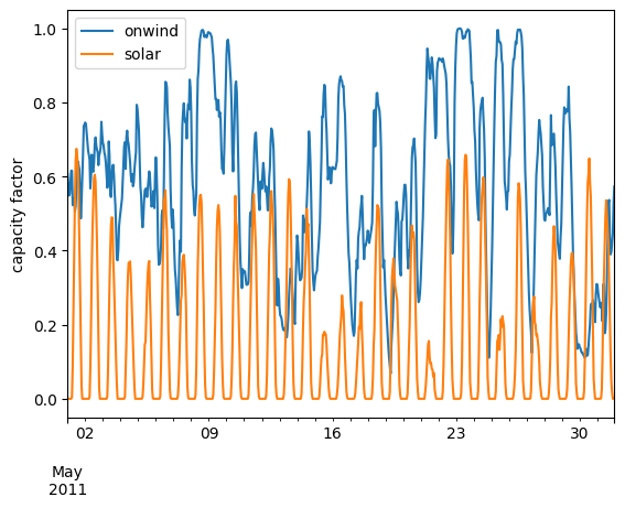
Task 4: Plot the wind and solar capacity factors for the month of May.
Show code cell content
Hide code cell content
df.loc["05-2011"].plot(ylabel="capacity factor")
<Axes: ylabel='capacity factor'>
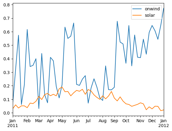
Task 5: Plot the weekly average capacity factors for wind and solar over the entire time period.
Show code cell content
Hide code cell content
df.resample("W").mean().plot()
<Axes: >
Task 6: Go to model.energy and retrieve the time series for another region of your choice. Recreate the analysis above and compare the results.
Note
Look for “Download Comma-Separated-Variable (CSV) file of data” in Step 2.