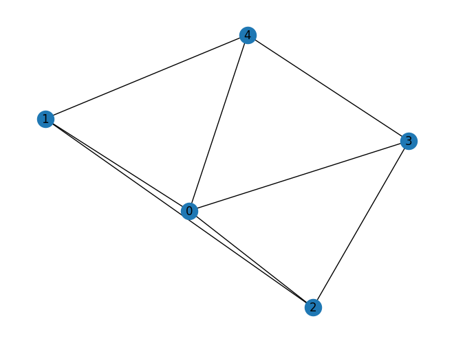
Solutions networkx

Exercise 1

Task 1: Build the graph shown above in networkx using the functions to add graphs. The weight of each edge should correspond to the sum of the node labels it connects.

Show code cell content

Hide code cell content

import networkx as nx

Show code cell content

Hide code cell content

G = nx.Graph()

Show code cell content

Hide code cell content

edges = [
    (0, 1, dict(weight=1)),
    (0, 2, dict(weight=2)),
    (0, 3, dict(weight=3)),
    (0, 4, dict(weight=4)),
    (1, 2, dict(weight=3)),
    (1, 4, dict(weight=5)),
    (2, 3, dict(weight=5)),
    (3, 4, dict(weight=7)),
]

Show code cell content

Hide code cell content

G.add_edges_from(edges)

Task 2: Draw the finished graph with matplotlib.

Show code cell content

Hide code cell content

nx.draw(G, with_labels=True)

Exercise 2

Reconsider the example of the European transmission network graph. Use the following code in a fresh notebook to get started:

url = "https://tubcloud.tu-berlin.de/s/FmFrJkiWpg2QcQA/download/edges.csv"
edges = pd.read_csv(url, index_col=0)

G = nx.from_pandas_edgelist(edges, "bus0", "bus1", edge_attr=["x_pu", "s_nom"])

subgraphs = []
for c in nx.connected_components(G):
    subgraphs.append(G.subgraph(c).copy())

Choose one of the subgraphs (each representing a synchronous zone) and perform the following analyses:

Show code cell content

Hide code cell content

import pandas as pd
import networkx as nx

url = "https://tubcloud.tu-berlin.de/s/FmFrJkiWpg2QcQA/download/edges.csv"
edges = pd.read_csv(url, index_col=0)

G = nx.from_pandas_edgelist(edges, "bus0", "bus1", edge_attr=["x_pu", "s_nom"])

subgraphs = []
for c in nx.connected_components(G):
    subgraphs.append(G.subgraph(c).copy())

Show code cell content

Hide code cell content

G = subgraphs[3]  # vary the subgraph here

Task 1: Determine the number of transmission lines and buses.

Show code cell content

Hide code cell content

len(G.edges)

408

Show code cell content

Hide code cell content

len(G.nodes)

286

Task 2: Check whether the network is planar.

Show code cell content

Hide code cell content

nx.is_planar(G)

False

Task 3: Calculate the average number of transmission lines connecting to a bus.

Show code cell content

Hide code cell content

pd.Series({k: v for k, v in G.degree}).mean()

np.float64(2.8531468531468533)

Task 4: Determine the number of cycles forming the cycle basis.

Show code cell content

Hide code cell content

len(nx.cycle_basis(G))

123

Task 5: Create a histogram of the length of the cycles (i.e. number of edges per cycle) in the cycle basis.

Show code cell content

Hide code cell content

cycle_length = pd.Series([len(c) for c in nx.cycle_basis(G)])

Show code cell content

Hide code cell content

cycle_length.plot.hist(bins=100);

Show code cell content

Hide code cell content

# alternative
pd.Series([len(c) for c in nx.cycle_basis(G)]).value_counts().sort_index().plot();

Task 6: Calculate the average length of the cycles in the cycle basis.

Show code cell content

Hide code cell content

cycle_length.describe()

count    123.000000
mean       8.918699
std        8.933813
min        3.000000
25%        3.000000
50%        5.000000
75%       11.000000
max       58.000000
dtype: float64

Task 7: Obtain the directed adjacency matrix.

Show code cell content

Hide code cell content

nx.adjacency_matrix(G).todense()

array([[0, 0, 0, ..., 0, 0, 0],
       [0, 0, 0, ..., 0, 0, 0],
       [0, 0, 0, ..., 0, 0, 0],
       ...,
       [0, 0, 0, ..., 0, 0, 0],
       [0, 0, 0, ..., 0, 0, 0],
       [0, 0, 0, ..., 0, 0, 0]], shape=(286, 286))

Task 8: Obtain the directed incidence matrix.

Show code cell content

Hide code cell content

K = nx.incidence_matrix(G).todense()
K

array([[1., 1., 0., ..., 0., 0., 0.],
       [0., 0., 1., ..., 0., 0., 0.],
       [0., 0., 0., ..., 0., 0., 0.],
       ...,
       [0., 0., 0., ..., 0., 0., 0.],
       [0., 0., 0., ..., 0., 0., 0.],
       [0., 0., 0., ..., 0., 0., 0.]], shape=(286, 408))