YouTube Video
Video not loading? Click here.
Why not pandas?
Let’s reload again our example dataset of conventional power plants in Europe as a pd.DataFrame.
import pandas as pd
import matplotlib.pyplot as plt

fn = "https://raw.githubusercontent.com/PyPSA/powerplantmatching/master/powerplants.csv"
exclude_carriers = ["Wind", "Solar", "Solid Biomass", "Biogas"]
ppl = pd.read_csv(fn, index_col=0).query(
    "Fueltype not in @exclude_carriers and Capacity > 20"
)
This dataset includes coordinates (latitude and longitude), which allows us to plot the location and capacity of all power plants in a scatter plot:
ppl.plot.scatter("lon", "lat", s=ppl.Capacity / 1e3)<Axes: xlabel='lon', ylabel='lat'>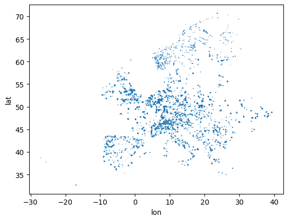
However, this graphs misses some geographic reference point, we’d normally expect for a map like shorelines, country borders and so on.
Why geopandas?

Geopandas extends pandas by adding support for geospatial data.
The core data structure in GeoPandas is the geopandas.GeoDataFrame, a subclass of pandas.DataFrame, that can store geometry columns and perform spatial operations.

Typical geometries are points, lines, and polygons. They come from another library called shapely, which helps you create, analyze, and manipulate two-dimensional shapes and their properties, such as points, lines, and polygons.
First, we need to import the geopandas package. The conventional alias is gpd:
import geopandas as gpdWe can convert the latitude and longitude values given in the dataset to formal geometries (to be exact, a shapely.Point object) using the gpd.points_from_xy() function, and use this to gpd.GeoDataFrame. We should also specify a so-called coordinate reference system (CRS). The code 4326 means latitude and longitude values, the so-called WGS84 system.
geometry = gpd.points_from_xy(ppl["lon"], ppl["lat"])
geometry[:5]
<GeometryArray>
[<POINT (9.925 51.899)>, <POINT (4.386 50.188)>, <POINT (9.88 47.085)>,
<POINT (6.581 45.204)>, <POINT (10.06 46.935)>]
Length: 5, dtype: geometrygdf = gpd.GeoDataFrame(ppl, geometry=geometry, crs=4326)Now, the resulting gdf looks like this:
gdf.head(3)gdf.geometry.head()id
0 POINT (9.92489 51.89857)
1 POINT (4.3862 50.1884)
2 POINT (9.88012 47.08503)
3 POINT (6.58145 45.2036)
4 POINT (10.05995 46.93529)
Name: geometry, dtype: geometryWith the additional geometry columns, it is now even easier to plot the geographic data:
gdf.plot(
    column="Fueltype",
    markersize=gdf.Capacity / 1e2,
)
<Axes: >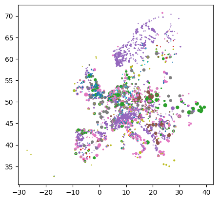
We can also start up an interactive map to explore the geodata in more detail:
gdf.explore(column="Fueltype")Projections with cartopy
Cartopy is a Python package designed for geospatial data processing and has an interface for handling projections in matplotlib maps.
Why is it needed?
The Earth is a globe, but we present maps usually on two-dimensional surfaces. Hence, we typically need to project data points onto flat surfaces (e.g. screens, paper). However, we will always loose some information in doing so.
A map projection is:
a systematic transformation of the latitudes and longitudes of locations from the surface of a sphere or an ellipsoid into locations on a plane. Wikipedia: Map projection.
Different projections preserve different metric properties. As a result, converting geodata from one projection to another is a common exercise in geographic data science.
conformal projections preserve angles/directions (e.g. Mercator projection)
equal-area projections preserve area measure (e.g. Mollweide)
equidistant projections preserve distances between points (e.g. Plate carrée)
compromise projections seek to strike a balance between distortions (e.g. Robinson)
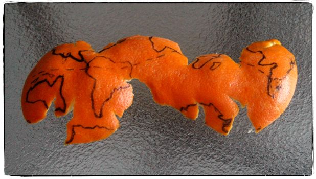
If you like the “Orange-as-Earth” analogy for projections, checkout this numberphile video by Hannah Fry.
First, we need to import the relevant parts of the cartopy package:
import cartopy
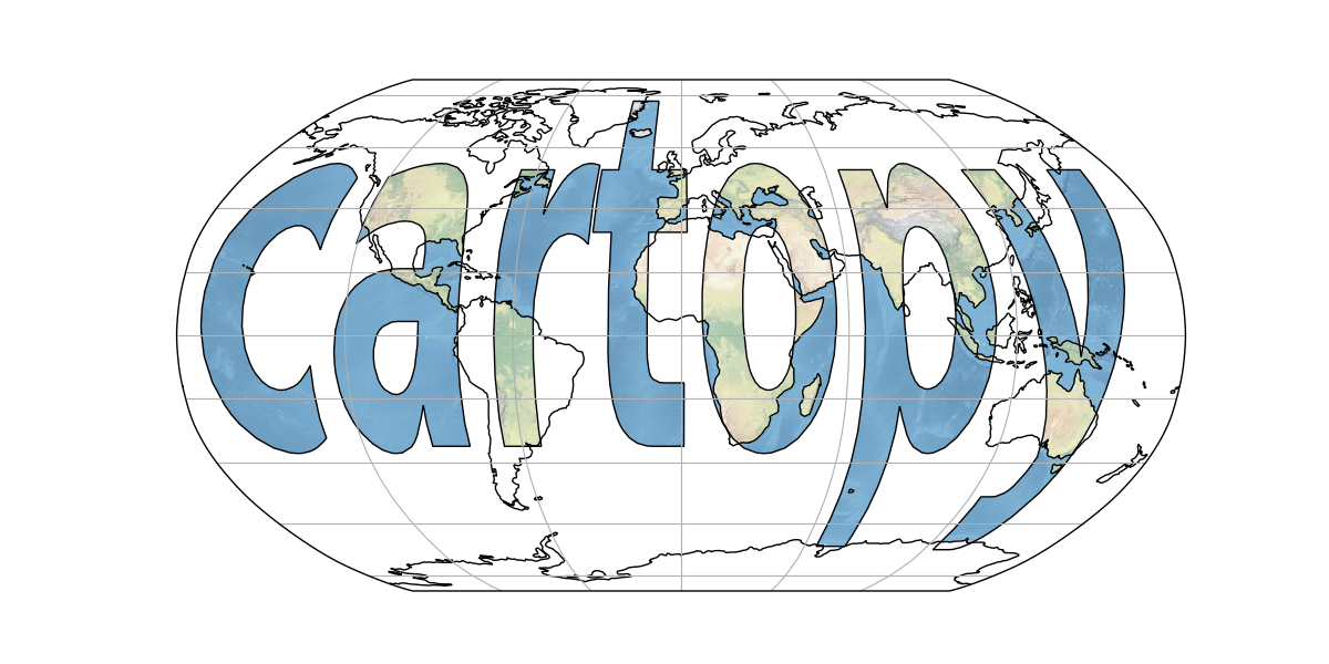
import cartopy.crs as ccrsLet’s draw a first map with cartopy outlining the global coastlines in the so-called plate carrée projection (equirectangular projection):
ax = plt.axes(projection=ccrs.PlateCarree())
ax.coastlines()
<cartopy.mpl.feature_artist.FeatureArtist at 0x7f5bc10d3770>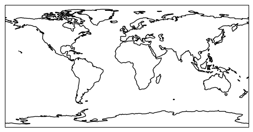
We can combine the functionality of cartopy with geopandas plots and even add geographical features:
fig = plt.figure(figsize=(7, 7))

ax = plt.axes(projection=ccrs.PlateCarree())

gdf.plot(
    ax=ax,
    column="Fueltype",
    markersize=gdf.Capacity / 1e2,
)

ax.coastlines()

ax.add_feature(cartopy.feature.BORDERS, color="red", linewidth=0.5)

ax.add_feature(cartopy.feature.OCEAN, color="blue")

ax.add_feature(cartopy.feature.LAND, color="yellow");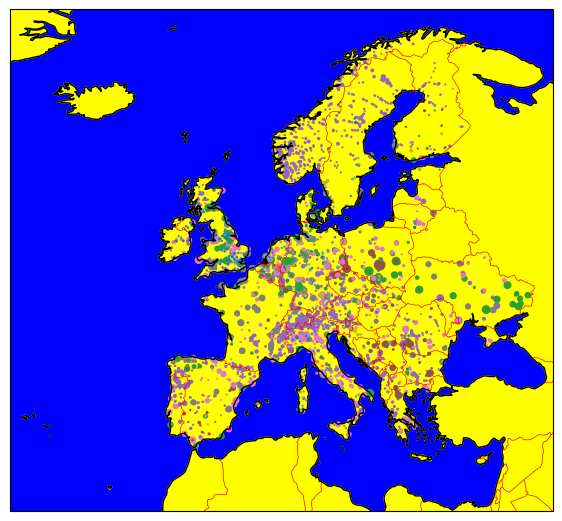
Geopandas will automatically calculate sensible bounds for the plot given the geographic data.
But we can also manually zoom in or out by setting the spatial extent with the .set_extent() method:
ax.set_extent([5, 16, 47, 55])
fig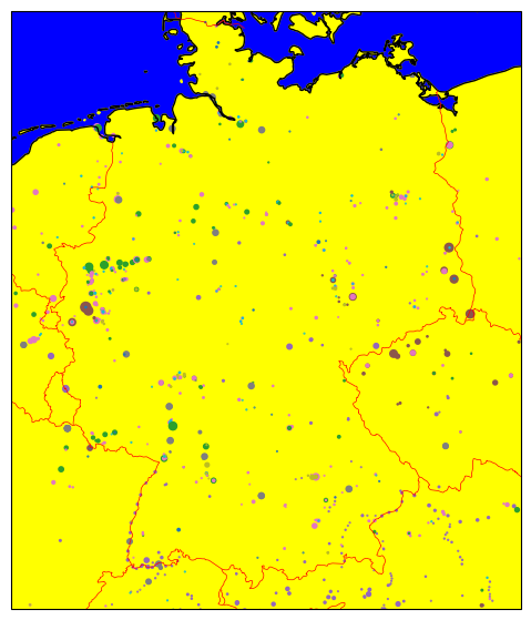
Reprojecting a GeoDataFrame
In geopandas, we can use the function .to_crs() to convert a GeoDataFrame with a given projection to another desired target coordinate reference system, using a cartopy CRS object:
crs = ccrs.Orthographic()
print(crs)
+proj=ortho +a=6378137.0 +lon_0=0.0 +lat_0=0.0 +alpha=0.0 +no_defs +type=crs
gdf.to_crs(crs).geometry.head()id
0 POINT (678339.313 5019080.88)
1 POINT (312316.755 4899390.89)
2 POINT (745194.941 4671124.57)
3 POINT (515078.664 4526021.742)
4 POINT (760750.157 4659758.366)
Name: geometry, dtype: geometryfig = plt.figure(figsize=(7, 7))
ax = plt.axes(projection=crs)
gdf.to_crs(crs).plot(
ax=ax,
column="Fueltype",
markersize=gdf.Capacity / 1e2,
)
ax.coastlines()<cartopy.mpl.feature_artist.FeatureArtist at 0x7f5bc196d810>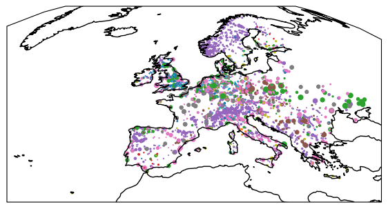
Reading and Writing Files
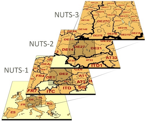
In the following example, we’ll load a dataset containing the NUTS regions:
Nomenclature of Territorial Units for Statistics or NUTS (French: Nomenclature des unités territoriales statistiques) is a geocode standard for referencing the subdivisions of countries for statistical purposes.
Our ultimate goal for this part of the tutorial is to map the power plant capacities to the NUTS-1 region they belong to.
Common filetypes for vector-based geospatial datasets are GeoPackage (.gpkg), GeoJSON (.geojson), File Geodatabase (.gdb), or Shapefiles (.shp).
In geopandas we can use the gpd.read_file() function to read such files. So let’s start:
url = "https://tubcloud.tu-berlin.de/s/RHZJrN8Dnfn26nr/download/NUTS_RG_10M_2021_4326.geojson"nuts = gpd.read_file(url)nuts.head(3)It is good practice to set an index. You can use .set_index() for that:
nuts = nuts.set_index("id")We can also check out the geometries in the dataset with .geometry:
nuts.geometryid
BG423 POLYGON ((24.42101 42.55306, 24.41032 42.4695,...
BG424 POLYGON ((25.07422 41.79348, 25.05851 41.75177...
BG425 POLYGON ((25.94863 41.32034, 25.90644 41.30757...
CH011 MULTIPOLYGON (((6.86623 46.90929, 6.89621 46.9...
CH012 POLYGON ((8.47767 46.5276, 8.39953 46.48872, 8...
...
LV POLYGON ((27.35158 57.51824, 27.54521 57.53444...
ME POLYGON ((20.06394 43.00682, 20.32958 42.91149...
MK POLYGON ((22.36021 42.31116, 22.51041 42.15516...
SK0 POLYGON ((19.88393 49.20418, 19.96275 49.23031...
IT MULTIPOLYGON (((12.47792 46.67984, 12.69064 46...
Name: geometry, Length: 2010, dtype: geometryWith .crs we can check in which coordinate reference system the data is given:
nuts.crs<Geographic 2D CRS: EPSG:4326>
Name: WGS 84
Axis Info [ellipsoidal]:
- Lat[north]: Geodetic latitude (degree)
- Lon[east]: Geodetic longitude (degree)
Area of Use:
- name: World.
- bounds: (-180.0, -90.0, 180.0, 90.0)
Datum: World Geodetic System 1984 ensemble
- Ellipsoid: WGS 84
- Prime Meridian: GreenwichWith .total_bounds we can check the bounding box of the data in the original coordinate reference system:
nuts.total_boundsarray([-63.08825, -21.38917, 55.83616, 80.76427])Let’s now filter the GeoDataFrame by NUTS-1 level...
nuts1 = nuts.query("LEVL_CODE == 1")... and explore what kind of geometries we have in the dataset ...
nuts1.explore()To write a GeoDataFrame back to file use GeoDataFrame.to_file(). The file format is inferred from the file ending.
nuts1.to_file("tmp.geojson")Buffers and Areas
Many geospatial analyses require the calculation of areas or buffers around geometries. However, these calculations depend on the coordinate reference system used.
The first thing we need to do in order to calculate area or buffers is to reproject the GeoDataFrame to an equal-area projection (here: EPSG:3035 which is valid only within Europe; a globally valid alternative is the Mollweide projection EPSG:54009)
nuts1 = nuts1.to_crs(3035)The area can be accessed via .area and is given in m² (after projection). Let’s convert to km²:
area = nuts1.area / 1e6
area.head()
id
AT1 23545.286205
AT2 25894.953057
EL4 17388.679384
EE0 45315.713593
EL3 3799.676547
dtype: float64nuts1.explore(column=area, vmax=1e5)We can also build a buffer of 1km around each geometry using .buffer():
nuts1.buffer(1000).explore()It is also possible to calculate the centroid of each geometry, which is the geometric center of a shape. It can be useful for labelling or constructing a point-based network representation of polygonal data:
ax = nuts1.geometry.plot()
nuts1.representative_point().plot(ax=ax, color="red", markersize=2)
<Axes: >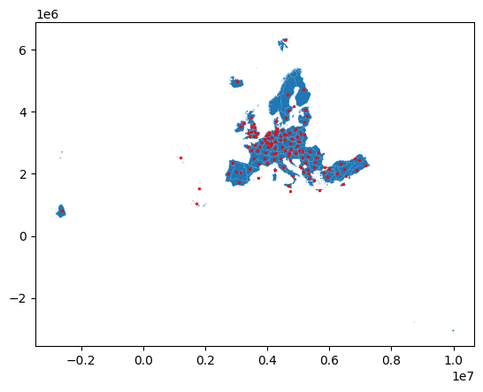
To calculate the distance between two points (or geometries more generally), we can use the .distance() method.
For instance, using the nuts1.representative_point() method, we can find a central point that represents each geometry but other than the centroid is guaranteed to be within the geometry. However, note that the distance is only meaningful if the geometries are in an appropriate projected coordinate reference system (e.g. an equidistant projection):
nuts1_de = nuts1.query("CNTR_CODE == 'DE'")
points = nuts1_de.representative_point()

ax = nuts1_de.plot()
points.plot(ax=ax, color="red", markersize=5)
<Axes: >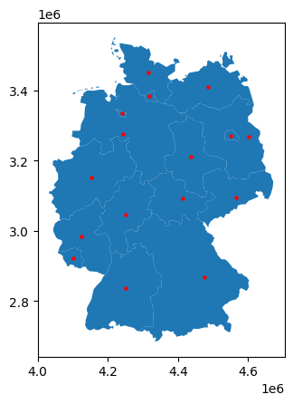
distances = (
    pd.concat({k: points.distance(p) for k, p in points.items()}, axis=1)
    .div(1e3)
    .astype(int)
)  # km
distancesThe .distance() function uses the haversine formula to calculate the great-circle distance between two points on the Earth’s surface, given their latitude and longitude coordinates.
Dissolve
The .dissolve() function is used to aggregate geometries within a GeoDataFrame based on a specified attribute or set of attributes. Practically, it is very similar to the pandas.DataFrame.groupby() function, but instead of aggregating numerical values, it merges geometries.
For instance, we can dissolve the NUTS regions by country code to get country-level geometries:
nuts1.dissolve("CNTR_CODE") # .plot()Spatial Joins
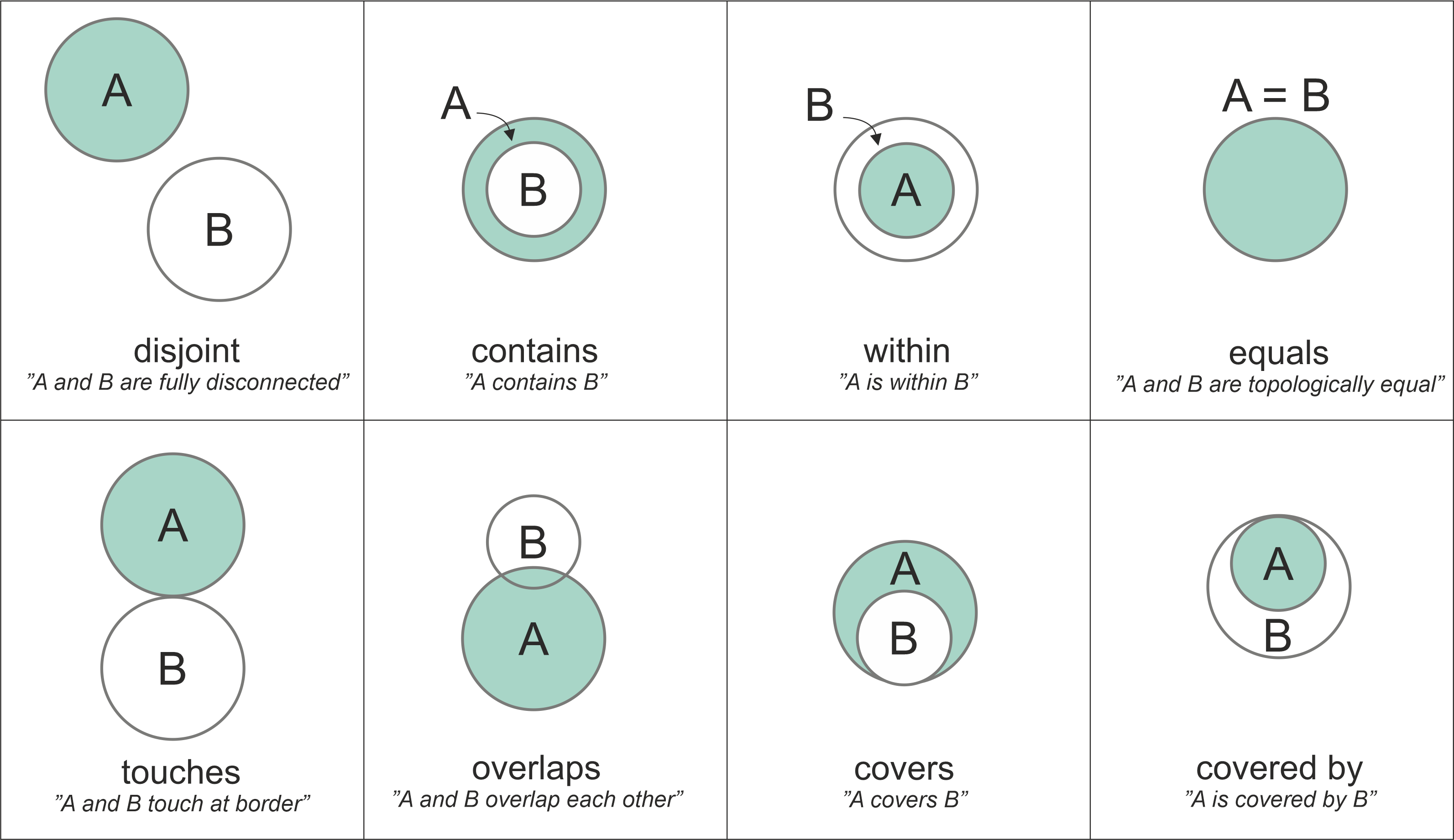
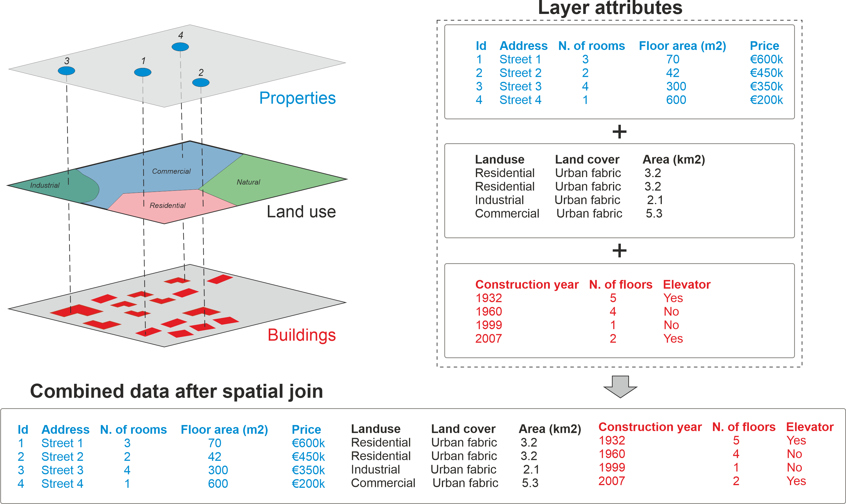
Multiple GeoDataFrames can be combined via spatial joins.
Observations from two datasets are combined with the .sjoin() function based on their spatial relationship to one another (e.g. whether they are intersecting, overlapping or contained within one another). You can read more about the specific options here.
Source: https://
To perform a spatial join, you need to provide the following information:
The two
geopandas.GeoDataFrameobjects you want to join (e.g.,left_dfandright_df).The type of spatial relationship to test (e.g.,
intersects,contains,within). This is specified using thepredicateparameter.The type of join to perform (e.g.,
inner,left,right). This is specified using thehowparameter. When usingleft, the resulting GeoDataFrame will retain all records from theleft_df, while matching records from theright_dfwill be added where the spatial relationship holds true. Withinner, only records with matches in both GeoDataFrames will be retained. Withright, all records from theright_dfwill be retained, with matching records from theleft_dfadded where applicable.
The .sjoin() function will then go through the geometries in both GeoDataFrames, evaluate the specified spatial relationship, and join the matching records (behind the scenes, it uses spatial indexing to speed up the process).
For example, if the predicate parameter is set to 'intersects', the function will check if the geometries of each record in left_df intersect with the geometries of any records in right_df. If a match is found, the attributes of the corresponding records from both GeoDataFrames will be combined into a new record in the output GeoDataFrame.
Source: https://
The result of the spatial join is a new GeoDataFrame that retains the geometries from the left_df and includes attributes from both GeoDataFrames for the matching records.
When no match is found, the resulting attributes from the right_df will be set to NaN (e.g. when some power plants are located outside of NUTS-1 regions).
Let’s do an example, starting with first reprojecting the gdf object of power plant to the same CRS as nuts1 polygons and reducing it to coal plants:
gdf = gdf.to_crs(3035).query("Fueltype == 'Nuclear'")Then, let’s have a look at both datasets at once. We want to find out which points (i.e. the power plants) lie within which shape (i.e. the NUTS1 regions).
fig = plt.figure(figsize=(7, 7))

ax = plt.axes(projection=ccrs.epsg(3035))

nuts1.plot(ax=ax, edgecolor="black", facecolor="sandybrown")

gdf.to_crs(3035).plot(
    ax=ax, column="Fueltype", markersize=gdf.Capacity / 40, legend=True
)

ax.set_extent([-7, 24, 40, 62])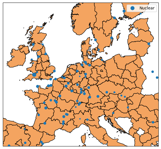
We can now apply the .sjoin() function. By default, .sjoin() looks for intersections and keeps the geometries of the left GeoDataFrame.
joined = gdf.sjoin(nuts1)If we look at this new GeoDataFrame, we now have additional columns from the NUTS1 data:
joined.head(3)We can now use these new columns for .groupby() operations on the capacities (as well as sorting, converting values to a suitable unit and renaming the index from NUTS identifiers to NUTS region names):
cap = joined.groupby("NUTS_ID").Capacity.sum().sort_values(ascending=False) / 1000  # GW
cap.rename(nuts1.NUTS_NAME).head(3)
NUTS_ID
Auvergne-Rhône-Alpes 15.927
Centre — Val de Loire 14.022
Grand Est 13.454
Name: Capacity, dtype: float64With our intersection and left join, some NUTS1 regions disappear in cap because they do not have any power plants. We can fix this by reindexing cap to the full set of NUTS1 regions:
nuts1.index.difference(cap.index)Index(['AL0', 'AT1', 'AT2', 'AT3', 'BE1', 'BG4', 'CY0', 'DE3', 'DE5', 'DE6',
'DE8', 'DEC', 'DED', 'DEE', 'DEG', 'DK0', 'EE0', 'EL3', 'EL4', 'EL5',
'EL6', 'ES1', 'ES2', 'ES3', 'ES6', 'ES7', 'FI1', 'FI2', 'FR1', 'FRC',
'FRG', 'FRL', 'FRM', 'FRY', 'HR0', 'HU1', 'HU3', 'IE0', 'IS0', 'ITG',
'LI0', 'LU0', 'LV0', 'ME0', 'MK0', 'MT0', 'NL1', 'NL3', 'NL4', 'NO0',
'PL2', 'PL4', 'PL5', 'PL6', 'PL7', 'PL8', 'PL9', 'PT1', 'PT2', 'PT3',
'RO1', 'RO3', 'RO4', 'RS1', 'RS2', 'SE2', 'SE3', 'TR1', 'TR2', 'TR3',
'TR4', 'TR5', 'TR6', 'TR7', 'TR8', 'TR9', 'TRA', 'TRB', 'TRC', 'UKE',
'UKF', 'UKG', 'UKI', 'UKJ', 'UKN'],
dtype='object')cap = cap.reindex(nuts1.index)
cap.head(3)id
AT1 NaN
AT2 NaN
EL4 NaN
Name: Capacity, dtype: float64Additionally, some power plants might be located outside of NUTS1 regions (e.g. the ones in Ukraine). Hence, the total capacity in cap is lower than the total capacity in gdf.
cap.sum() < gdf.Capacity.div(1e3).sum()np.True_Finally, we can plot the total hard coal generation capacity per NUTS1 region on a map.
For regions without any coal power plants we can use the missing_kwds parameter to set a specific appearance (here red hatching).
fig = plt.figure(figsize=(7, 7))

ax = plt.axes(projection=ccrs.epsg(3035))

nuts1.plot(
    ax=ax,
    column=cap,
    legend=True,
    missing_kwds={
        "color": "lightgrey",
        "edgecolor": "red",
        "hatch": "///",
    },
    legend_kwds={"label": "Hard Coal Capacity [GW]", "shrink": 0.7},
)

ax.set_extent([-7, 24, 40, 62])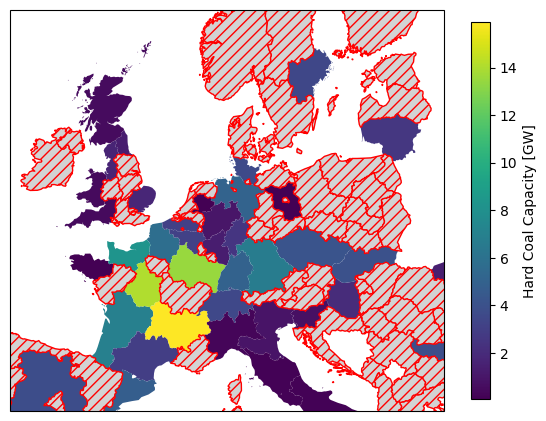
This concludes the geopandas and cartopy tutorial!
Exercises
Take the following code snippet as a starting point. It loads the NUTS regions of Europe, the power plant dataset, and a shapefile for the Danish Natura2000 natural protection areas.
import cartopy
import pandas as pd
import geopandas as gpd
import cartopy.crs as ccrs
import matplotlib.pyplot as plt

url = "https://tubcloud.tu-berlin.de/s/RHZJrN8Dnfn26nr/download/NUTS_RG_10M_2021_4326.geojson"
nuts = gpd.read_file(url)

fn = "https://raw.githubusercontent.com/PyPSA/powerplantmatching/master/powerplants.csv"
df = pd.read_csv(fn, index_col=0)
geometry = gpd.points_from_xy(df["lon"], df["lat"])
ppl = gpd.GeoDataFrame(df, geometry=geometry, crs=4326)

url = "https://tubcloud.tu-berlin.de/s/mEpdmgBtmMbyjAr/download/Natura2000_end2021-DK.gpkg"
natura = gpd.read_file(url)
Task 1: Identify the coordinate reference system of the natura GeoDataFrame.
Task 2: Plot the natura GeoDataFrame on a map without transforming its CRS. Use cartopy for setting the projection of the figure and add coastlines and borders.
Task 3: Identify the name of the largest protected area in the natura GeoDataFrame.
Task 4: What is the total protection area in square kilometers.
Task 5: The natura GeoDataFrame has a column SITETYPE that indicates the type of protected area. Calculate the total area for each type of protected area (again in square kilometers).
Task 6: By how much (in percent) would the total area of protected areas increase if a buffer of 1 km around each protected area were also protected?
Task 7: List the power plants that are located within protected areas. How many power plants are located within protected areas? Use the .sjoin() function. Check the result by plotting these power plants on top of the protected areas.
Task 8 (advanced): What fraction of the natural protection area is located offshore? Use set operations with the .overlay() function and the NUTS regions GeoDataFrame.