Group Work Preparation - Data Science for Energy System Modelling

This tutorial contains various small guides for tasks will come in handy in the upcoming group assignment:

Downloading historical weather data with atlite from ERA5.
Working with representative points in geopandas and calculating crow-fly distances.
Setting up the Gurobi solver for optimisation problems (optional).

import atlite
import pypsa
import geopandas as gpd
import pandas as pd
import matplotlib.pyplot as plt
from urllib.request import urlretrieve

ERA5 Data Download¶

Suppose you have chosen the Netherlands as your case study region and want to download historical weather data for 1 March 2013 from the ERA5 dataset.

fn = "https://tubcloud.tu-berlin.de/s/567ckizz2Y6RLQq/download?path=%2Fgadm&files=gadm_410-levels-ADM_1-NLD.gpkg"
regions = gpd.read_file(fn)
regions.plot()

<Axes: >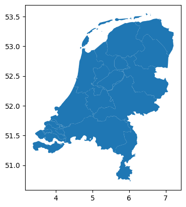

You can use the atlite package to handle requests to download from the Copernicus Climate Data Store (CDS) which provides the ERA5 data, so that you don’t have to manually go through the CDS web interface.

Before you can start, you need to set up an account at the Copernicus Climate Data Store and get an API key.

An API key is a unique identifier of your account and a way to authenticate users when accessing the CDS programmatically. It is typically stored in a configuration file (i.e., .cdsapirc in your home directory for the CDS API).

The setup instructions for the CDS API differ by operating system and can be found on the CDS API page. When you are logged in, your personal API key will be shown:

url: https://cds.climate.copernicus.eu/api
key: <PERSONAL-ACCESS-TOKEN>

Note that before you can start downloading data, you need to accept the terms of use of the ERA5 dataset here (while logged in). You do not need to run any API requests from the web interface! This will be done via atlite.

Once you have set up your account and API key, you can start using atlite to create a cutout and download the data you need.

Remember that a cutout in atlite defines the spatial and temporal extent of the weather data you want to work with.

A cutout is loaded or created under path provided via the path keyword of atlite.Cutout; the behaviour varies whether the cutout already exists or not:

If a cutout already exists at the path, a call to atlite.Cutout() will simply load the cutout again from the hard drive and not try to connect to the CDS API.
If the cutout does not yet exist, a call to atlite.Cutout() specifies the target file for a new cutout to be created by downloading from the CDS API.

For creating a cutout, next to the path, you need to specify the dataset module (here: ERA5), a time period under time, and the spatial extent (in latitude y and longitude x).

For our example of the Netherlands, we first access the spatial bounds of the country shape and add a 0.25 degree buffer (approximately one grid cell) around it:

minx, miny, maxx, maxy = regions.total_bounds
buffer = 0.25

cutout = atlite.Cutout(
    path="era5-2013-03-NL.nc",
    module="era5",
    x=slice(minx - buffer, maxx + buffer),
    y=slice(miny - buffer, maxy + buffer),
    time="2013-03-01",
)

Once the cutout is defined, calling the function cutout.prepare() initiates the connection to the CDS API, the download and pre-processing of the weather data. Because the download needs to be provided by the CDS servers, this might take a while depending on the amount of data requested and the length of the queue.

# cutout.prepare(compression=None)

If we have another cutout prepared (like from the URL below), atlite will simply load the cutout from disk instead of downloading it again:

fn = "era5-2013-NL.nc"
url = "https://tubcloud.tu-berlin.de/s/bAJj9xmN5ZLZQZJ/download/" + fn
urlretrieve(url, fn);

cutout2 = atlite.Cutout(path=fn)
cutout2

/home/runner/work/data-science-for-esm/data-science-for-esm/.venv/lib/python3.13/site-packages/xarray/backends/plugins.py:109: RuntimeWarning:

Engine 'cfgrib' loading failed:
Cannot find the ecCodes library

<Cutout "era5-2013-NL">
 x = 3.25 ⟷ 7.25, dx = 0.25
 y = 50.50 ⟷ 53.75, dy = 0.25
 time = 2013-01-01 ⟷ 2013-12-31, dt = h
 module = era5
 prepared_features = ['height', 'wind', 'influx', 'temperature', 'runoff']

Global Equal-Area and Equal-Distance CRS¶

Previously, we used EPSG:3035 as projection to calculate the area of regions in km². However, this projection is not correct for regions outside of Europe, so that we need to pick different, more suitable projections for calculating areas and distances in non-European regions. There are two good options for global projections that preserve either distances or areas:

for calculating distances: WGS 84 / World Equidistant Cylindrical (EPSG:4087)
for calculating areas: Mollweide (ESRI:54009)

The unit of measurement for both projections is metres.

AREA_CRS = "ESRI:54009"
DISTANCE_CRS = "EPSG:4087"

world = gpd.read_file(
    "https://naciscdn.org/naturalearth/110m/cultural/ne_110m_admin_0_countries.zip"
)

world.to_crs(AREA_CRS).plot()

<Axes: >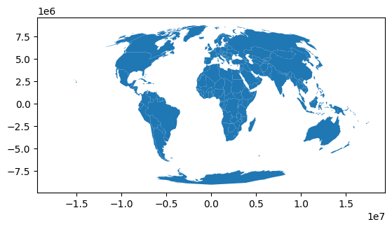

world.to_crs(DISTANCE_CRS).plot()

<Axes: >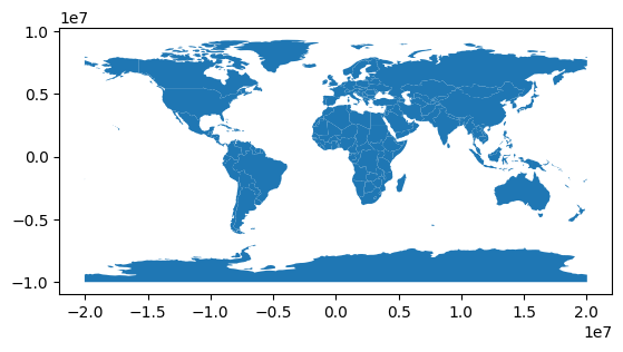

Representative Points and Crow-Fly Distances¶

The following example includes code to retrieve representative points from polygons and to calculate the distance on a sphere between two points. This can be useful when calculating approximate distances for transmission lines between two regions.

world = gpd.read_file(
    "https://naciscdn.org/naturalearth/110m/cultural/ne_110m_admin_0_countries.zip"
)

points = world.representative_point()

fig, ax = plt.subplots()
world.plot(ax=ax)
points.plot(ax=ax, color="red", markersize=3);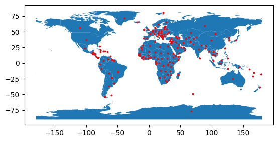

points = points.to_crs(4087)
points.index = world.ISO_A3

distances = pd.concat({k: points.distance(p) for k, p in points.items()}, axis=1).div(
    1e3
)  # km

distances.loc["DEU", "NLD"]

np.float64(564.4945392494385)

Gurobi Solver Setup¶

Gurobi is one of the fastest solvers to solve optimisation problems. It is a commercial solver, with free academic licenses.

Using this solver for the group assignment is optional. You can also use other open-source alternatives, but they might take longer to solve or do not converge for larger problems.

To set up Gurobi, you need to:

Install the Gurobi Python package gurobipy inside your environment. Use pip install gurobipy or conda install -c gurobi gurobi with your environment already activated.
Register at here with your institutional e-mail address (e.g. @campus.tu-berlin.de).
Request an academic license here (while logged in) from within the university network or via VPN. Choose the Named-User Academic license type.
You will get pop-up instructions to run a command (e.g., grbgetkey abcdef-1234-5678-abcd-abcdef123456) in your terminal to activate the license. Copy and paste this command into your terminal and run it.

That should be it! You can now use Gurobi as solver with PyPSA:

n = pypsa.examples.ac_dc_meshed()
# n.optimize(solver_name='gurobi')

INFO:pypsa.network.io:Retrieving network data from https://github.com/PyPSA/PyPSA/raw/v1.0.6/examples/networks/ac-dc-meshed/ac-dc-meshed.nc.

INFO:pypsa.network.io:New version 1.0.7 available! (Current: 1.0.6)

INFO:pypsa.network.io:Imported network 'AC-DC-Meshed' has buses, carriers, generators, global_constraints, lines, links, loads

On this online website, Gurobi is not installed, so PyPSA will complain with AssertionError: Solver gurobi not installed.