NetworkX

NetworkX: Network Analysis in Python

NetworkX is a Python package for the creation, manipulation, and study of the structure, dynamics, and functions of complex networks.

Mainly, networkx provides data structures for undirected and directed graphs as well as multigraphs (graphs with multiple edges between nodes) for which many standard graph algorithms are implemented (such as shortest paths, clustering, cycle detection, and more).

Note

If you have not yet set up Python on your computer, you can execute this tutorial in your browser via Google Colab. Download the .ipynb file using the download button on the top right corner and import it in Google Colab.

Then install the following packages by executing the following command in a Jupyter cell at the top of the notebook.

!pip install numpy networkx pandas matplotlib

Let’s perform some network analysis on this simple graph:

Simple Graphs¶

import numpy as np

Say we want to calculate the so-called Laplacian $L$ of this graph based on its incidence matrix $K$ , which is an $N\times N$ matrix defined as $L=KK^\top$ for an undirected graph. The Laplacian matrix of a graph is a representation that captures the connectivity and structure of the graph by quantifying the difference between the degree of each vertex and the adjacency relationships with its neighbouring vertices. We first need to write down the incidence matrix $K$ as a np.array. Let’s also use the convention that edges are oriented such that they are directed at the node with the higher label value (i.e. from node 1 to node 2, not vice versa).

K = np.array(
    [
        [1, -1, 0, 0],
        [1, 0, -1, 0],
        [0, 1, -1, 0],
        [0, 0, 1, -1],
    ]
).T
K

array([[ 1,  1,  0,  0],
       [-1,  0,  1,  0],
       [ 0, -1, -1,  1],
       [ 0,  0,  0, -1]])

L = K.dot(K.T)
L

array([[ 2, -1, -1,  0],
       [-1,  2, -1,  0],
       [-1, -1,  3, -1],
       [ 0,  0, -1,  1]])

This is all fine for small graphs, but inconvient for larger graphs. Let’s take the help from networkx!

The `Graph` object¶

First, let’s import the library. It is commonly imported under the alias nx.

import networkx as nx

This is how we can create an empty graph with no nodes and no edges.

G = nx.Graph()

Nodes¶

We can add one node at a time,

G.add_node(1)

with attributes

G.add_node(2, country="DE")

or add nodes from a list

G.add_nodes_from([3, 4])

We can also add nodes along with node attributes if your container yields 2-tuples of the form (node, node_attribute_dict):

G.add_nodes_from(
    [
        (5, {"color": "red"}),
        (6, {"color": "green"}),
    ]
)

Edges¶

G can also be grown by adding one edge at a time,

G.add_edge(1, 2)

even with attributes

G.add_edge(3, 4, weight=2)

or by adding a list of edges,

G.add_edges_from([(1, 3), (2, 5)])

or as a 3-tuple with 2 nodes followed by an edge attribute dictionary

G.add_edges_from([(2, 3, {"weight": 3})])

Examining elements of a graph¶

We can examine the nodes and edges.

G.nodes

NodeView((1, 2, 3, 4, 5, 6))

G.number_of_nodes()

6

G.edges

EdgeView([(1, 2), (1, 3), (2, 5), (2, 3), (3, 4)])

G.number_of_edges()

5

Accessing graph elements¶

Access an edge:

G.edges[2, 3]

{'weight': 3}

Access an attribute of an edge:

G.edges[2, 3]["weight"]

3

Find all neighbours of node 1:

G[1]

AtlasView({2: {}, 3: {}})

Removing elements¶

One can remove nodes and edges from the graph in a similar fashion to adding. Use methods G.remove_node(), G.remove_nodes_from(), G.remove_edge() and G.remove_edges_from(), e.g.

G.remove_node(5)

try:
    G.remove_edge(2, 5)
except Exception as e:
    print(e)

The edge 2-5 is not in the graph

You can remove all nodes and edges with

# G.clear()

Visualising graphs¶

A basic drawing function for networks is also available in networkx

nx.draw(G)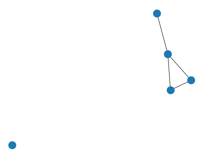

with options for labeling graph elements

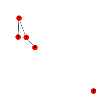
nx.draw(G, with_labels=True)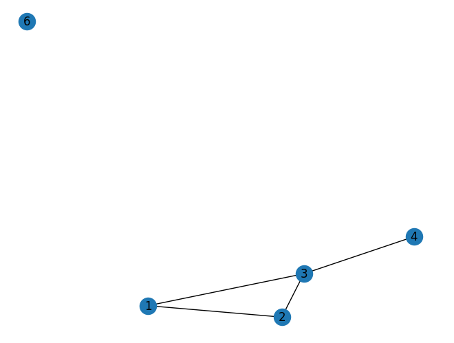

and integration to matplotlib

import matplotlib.pyplot as plt

fig, ax = plt.subplots(figsize=(5, 5))
nx.draw(G, with_labels=True, ax=ax, node_color="green", font_weight="bold")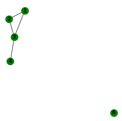

Analysing graphs¶

The networkx library comes with many functions to analyse graphs. Here are a few examples we’re going to need for linearised power flow calculations in electricity transmission networks:

Are all nodes in the network connected with each other?

nx.is_connected(G)

False

What are the components that are connected / isolated?

list(nx.connected_components(G))

[{1, 2, 3, 4}, {6}]

Is the network planar? I.e. can the graph be drawn such that edges don’t cross?

nx.is_planar(G)

True

What is the frequency of degrees in the network?

nx.degree_histogram(G)

[1, 1, 2, 1]

import pandas as pd

pd.Series(nx.degree_histogram(G))

0    1
1    1
2    2
3    1
dtype: int64

What is the adjacency matrix? (Careful, networkx will yield a weighted adjacency matrix by default!)

A = nx.adjacency_matrix(G, weight=None).todense()
A

array([[0, 1, 1, 0, 0],
       [1, 0, 1, 0, 0],
       [1, 1, 0, 1, 0],
       [0, 0, 1, 0, 0],
       [0, 0, 0, 0, 0]])

What is the incidence matrix? (Careful, networkx will yield a incidence matrix without orientation by default!)

nx.incidence_matrix(G, oriented=True).todense()

array([[-1., -1.,  0.,  0.],
       [ 1.,  0., -1.,  0.],
       [ 0.,  1.,  1., -1.],
       [ 0.,  0.,  0.,  1.],
       [ 0.,  0.,  0.,  0.]])

What is the Laplacian matrix? (Careful, networkx will yield a weighted adjacency matrix by default!)

L = nx.laplacian_matrix(G, weight=None).todense()
L

array([[ 2, -1, -1,  0,  0],
       [-1,  2, -1,  0,  0],
       [-1, -1,  3, -1,  0],
       [ 0,  0, -1,  1,  0],
       [ 0,  0,  0,  0,  0]])

Find a cycle basis (i.e. a collection of independent cycles through which all other cycles can be represented through linear combination):

nx.cycle_basis(G)

[[1, 2, 3]]

This function returns a list of sequences. Each sequence indicates a series of nodes to traverse for the respective cycle.

Example: European Transmission Network¶

Let’s now apply what we have learned to a real-world example. In this example, we are going to load a slightly simplified dataset of the European high-voltage transmission network. In this dataset, HVDC links and back-to-back converters have been left out, and the data only shows AC transmission lines.

url = "https://tubcloud.tu-berlin.de/s/898dEKqG6XEDqqS/download/nodes.csv"
nodes = pd.read_csv(url, index_col=0)
nodes.head(5)

url = "https://tubcloud.tu-berlin.de/s/FmFrJkiWpg2QcQA/download/edges.csv"
edges = pd.read_csv(url, index_col=0)
edges.head(5)

networkx provides a utility function nx.from_pandas_edgelist() to build a network from edges listed in a pandas.DataFrame:

N = nx.from_pandas_edgelist(edges, "bus0", "bus1", edge_attr=["x_pu", "s_nom"])

We can get some basic info about the graph:

print(N)

Graph with 3532 nodes and 5157 edges

pd.Series(nx.degree_histogram(N)).plot.bar()
plt.xlabel("Degree (number of connections)")
plt.ylabel("Number of nodes")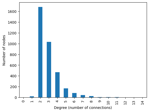

degrees = [val for node, val in N.degree()]
np.mean(degrees)

np.float64(2.920158550396376)

The nodes DataFrame provides us with the coordinates of the graph’s nodes. To make the nx.draw() function use these coordinates, we need to bring them into a particular format.

{nodeA: (x, y),
 nodeB: (x, y),
 nodeC: (x, y)}

pos = nodes.apply(tuple, axis=1).to_dict()

Let’s just look at the first 5 elements of the dictionary to check:

{k: pos[k] for k in list(pos.keys())[:5]}

{8838: (-2.16979999999999, 53.243852),
 7157: (11.9273472385104, 45.403085502256),
 1316: (14.475861, 40.761821),
 7421: (4.52012724307074, 50.4886188621382),
 1317: (14.639282, 40.688969)}

Now, we can draw the European transmission network:

fig, ax = plt.subplots(figsize=(10, 10))
nx.draw(N, pos=pos, node_size=0)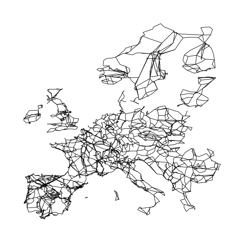

You can already see that not all parts of the Network are connected with each other. Ireland, Great Britain, Scandinavia, and some Islands in the Mediterranean are not connected to the continental grid. At least not via AC transmission lines. They are through HVDC links and back-to-back converters. These subgraphs denote the different synchronous zones of the European transmission network:

len(list(nx.connected_components(N)))

7

Let’s build subgraphs for the synchronous zones by iterating over the connected components:

subgraphs = []
for c in nx.connected_components(N):
    subgraphs.append(N.subgraph(c).copy())

We can now color-code them in the network plot:

fig, ax = plt.subplots(figsize=(10, 10))
colors = ["red", "blue", "green", "orange", "teal", "cyan", "black"]
for i, sub in enumerate(subgraphs):
    sub_pos = {k: v for k, v in pos.items() if k in sub.nodes}
    nx.draw(sub, pos=sub_pos, node_size=0, edge_color=colors[i])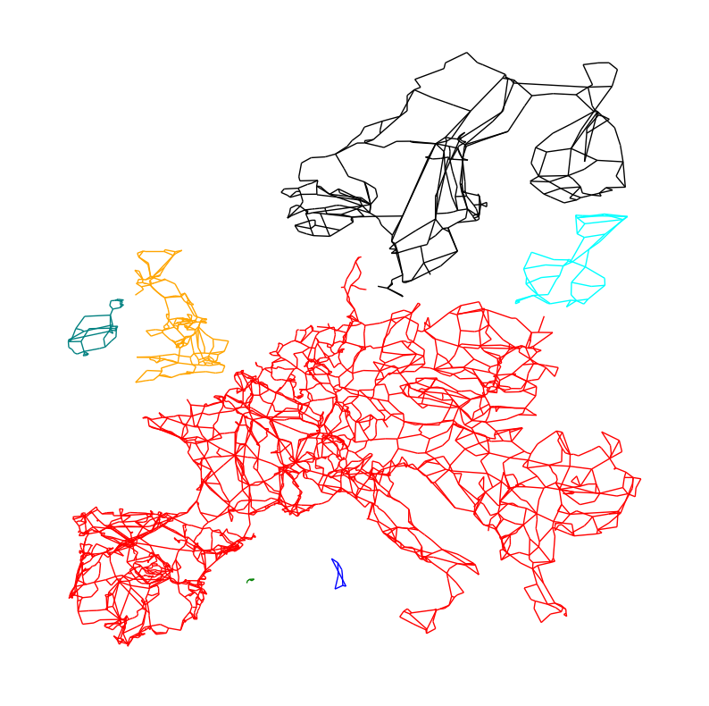

Exercises¶

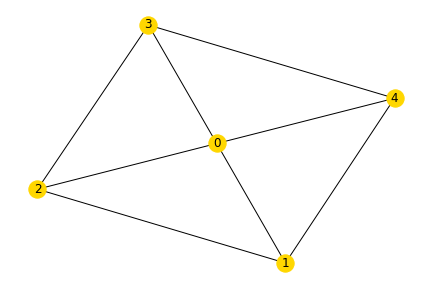
Exercise 1¶

Task 1: Build the following graph in networkx using the functions to add graphs. The weight of each edge should correspond to the sum of the node labels it connects.

Task 2: Draw the finished graph with matplotlib.

Exercise 2¶

Reconsider the example of the European transmission network graph. Use the following code in a fresh notebook to get started:

url = "https://tubcloud.tu-berlin.de/s/FmFrJkiWpg2QcQA/download/edges.csv"
edges = pd.read_csv(url, index_col=0)

G = nx.from_pandas_edgelist(edges, "bus0", "bus1", edge_attr=["x_pu", "s_nom"])

subgraphs = []
for c in nx.connected_components(G):
    subgraphs.append(G.subgraph(c).copy())

Choose one of the subgraphs (each representing a synchronous zone) and perform the following analyses:

Task 1: Determine the number of transmission lines and buses.

Task 2: Check whether the network is planar.

Task 3: Calculate the average number of transmission lines connecting to a bus.

Task 4: Determine the number of cycles forming the cycle basis.

Task 5: Create a histogram of the length of the cycles (i.e. number of edges per cycle) in the cycle basis.

Task 6: Calculate the average length of the cycles in the cycle basis.

Task 7: Obtain the directed adjacency matrix.

Task 8: Obtain the directed incidence matrix.

Simple Graphs¶

The Graph object¶

Nodes¶

Edges¶

Examining elements of a graph¶

Accessing graph elements¶

Removing elements¶

Visualising graphs¶

Analysing graphs¶

Example: European Transmission Network¶

Exercises¶

Exercise 1¶

Exercise 2¶

The `Graph` object¶