Pandas

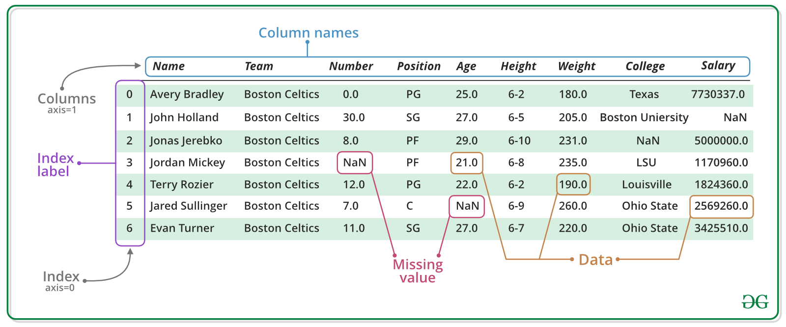
Pandas is a an open source library providing Excel-like tables in Python. It offers functionality for efficiently reading, writing, and processing data such as sorting, filtering, aggregating, and visualizing. Moreover, it provides tools for handling missing data and time series data.

Note

If you have not yet set up Python on your computer, you can execute this tutorial in your browser via Google Colab. Download the .ipynb file using the download button on the top right corner and import it in Google Colab.

Then install pandas and numpy by executing the following command in a Jupyter cell at the top of the notebook.

!pip install pandas numpy

import pandas as pd
import numpy as np

The `Series`¶

A Series represents a one-dimensional array of data. The main difference between a Series and numpy array is that a Series has an index. The index contains the labels that we use to access the data. It is actually quite similar to a Python dictionary, where each value is associated with a key.

There are many ways to create a Series, but the core constructor is pd.Series() which can process a dictionary to create a Series.

dictionary = {
    "Neckarwestheim": 1269,
    "Isar 2": 1365,
    "Emsland": 1290,
}
s = pd.Series(dictionary)
s

Neckarwestheim    1269
Isar 2            1365
Emsland           1290
dtype: int64

dictionary

{'Neckarwestheim': 1269, 'Isar 2': 1365, 'Emsland': 1290}

Arithmetic operations and most numpy functions can be applied to pd.Series. An important point is that the Series keep their index during such operations.

np.log(s) / s**0.5

Neckarwestheim    0.200600
Isar 2            0.195391
Emsland           0.199418
dtype: float64

We can access the underlying index object if we need to:

s.index

Index(['Neckarwestheim', 'Isar 2', 'Emsland'], dtype='object')

We can get values back out using the index via the .loc attribute

s.loc["Isar 2"]

np.int64(1365)

Or by raw position using .iloc

s.iloc[2]

np.int64(1290)

We can pass a list or array to loc to get multiple rows back:

s.loc[["Neckarwestheim", "Emsland"]]

Neckarwestheim    1269
Emsland           1290
dtype: int64

And we can even use so-called slicing notation (:) to get ranges of rows:

s.loc["Neckarwestheim":"Emsland"]

Neckarwestheim    1269
Isar 2            1365
Emsland           1290
dtype: int64

s.iloc[:2]

Neckarwestheim    1269
Isar 2            1365
dtype: int64

If we need to, we can always get the raw data back out as well

type(s.values)  # a numpy array

numpy.ndarray

The `DataFrame`¶

There is a lot more to a pandas.Series, but they are limit to a single column. A more broadly useful Pandas data structure is the DataFrame. pandas.DataFrame is a collection of series that share the same index. It’s a lot like a table in a spreadsheet.

The core constructor is pd.DataFrame(), which can be used like this using a dictionary of lists:

data = {
    "capacity": [1269, 1365, 1290],  # MW
    "type": ["PWR", "PWR", "PWR"],
    "start_year": [1989, 1988, 1988],
    "end_year": [np.nan, np.nan, np.nan],
}

df = pd.DataFrame(data, index=["Neckarwestheim", "Isar 2", "Emsland"])
df

We can also switch columns and rows very easily using the .T (transpose) attribute:

df

A wide range of statistical functions are available on both Series and DataFrames.

df.min()

capacity      1269
type           PWR
start_year    1988
end_year       NaN
dtype: object

df.mean(numeric_only=True)

capacity      1308.000000
start_year    1988.333333
end_year              NaN
dtype: float64

df.describe()

We can get a single column as a Series using python’s getitem syntax on the DataFrame object.

df["capacity"]

Neckarwestheim    1269
Isar 2            1365
Emsland           1290
Name: capacity, dtype: int64

...or using attribute syntax.

df.end_year

Neckarwestheim   NaN
Isar 2           NaN
Emsland          NaN
Name: end_year, dtype: float64

Indexing works very similar to series

df.loc["Emsland"]

capacity      1290
type           PWR
start_year    1988
end_year       NaN
Name: Emsland, dtype: object

df.iloc[2]

capacity      1290
type           PWR
start_year    1988
end_year       NaN
Name: Emsland, dtype: object

But we can also specify the column(s) and row(s) we want to access

df.loc["Emsland", "start_year"]

np.int64(1988)

df.loc[["Emsland", "Neckarwestheim"], ["start_year", "end_year"]]

Mathematical operations work as well, either on the whole DataFrame or on specific columns, the result of which can be assigned to a new column:

df.capacity * 0.8

Neckarwestheim    1015.2
Isar 2            1092.0
Emsland           1032.0
Name: capacity, dtype: float64

df["reduced_capacity"] = df.capacity * 0.8
df

Cleaning Data¶

We can also remove columns or rows from a DataFrame:

df.drop("reduced_capacity", axis="columns")
df

We can update the variable df by either overwriting df or passing an inplace keyword:

df = df.drop("reduced_capacity", axis="columns")

df

We can also drop columns with only NaN values

df.dropna(axis=1, how="any")

Or fill it up with default fallback data:

df.fillna(2023)
df

Say, we already have one value for end_year and want to fill up the missing data. We can use forward fill (ffill) or backward fill (bfill):

df.loc["Emsland", "end_year"] = 2023
df.loc["Neckarwestheim", "end_year"] = 2026
df

df["end_year"] = df["end_year"].ffill()
df
df["x"] = np.nan
df["y"] = np.nan
df

Sometimes it can be useful to rename columns:

df.rename(columns=dict(x="lat", y="lon"))

Sometimes it can be useful to replace values:

df.replace({"PWR": "Pressurized water reactor"})

df

In many cases, we want to modify values in a dataframe based on some rule. To modify values, we need to use .loc or .iloc. It can be use to set a specific value or a set of values based on their index and column labels:

df.loc["Isar 2", "start_year"] = 2000
df.loc["Emsland", "capacity"] += 10
df

It can even be a completely new column:

operational = ["Neckarwestheim", "Isar 2", "Emsland"]
df.loc[operational, "y"] = [49.04, 48.61, 52.47]
df

Combining Datasets¶

Pandas supports a wide range of methods for merging different datasets. These are described extensively in the documentation. Here we just give a few examples.

data = {
    "capacity": [1288, 1360, 1326],  # MW
    "type": ["BWR", "PWR", "PWR"],
    "start_year": [1985, 1985, 1986],
    "end_year": [2021, 2021, 2021],
    "x": [10.40, 9.41, 9.35],
    "y": [48.51, 52.03, 53.85],
}
df2 = pd.DataFrame(data, index=["Gundremmingen", "Grohnde", "Brokdorf"])
df2

We can now add this additional data to the df object

df = pd.concat([df, df2])
df

Sorting & Filtering Data¶

We can also sort the entries in dataframes, e.g. alphabetically by index or numerically by column values

df.sort_index()

df.sort_values(by="end_year", ascending=False)

We can also filter a DataFrame using a boolean series obtained from a condition. This is very useful to build subsets of the DataFrame.

df.capacity > 1300

Neckarwestheim    False
Isar 2             True
Emsland           False
Gundremmingen     False
Grohnde            True
Brokdorf           True
Name: capacity, dtype: bool

df[df.capacity > 1300]

We can also combine multiple conditions, but we need to wrap the conditions with brackets!

df[(df.capacity > 1300) & (df.start_year >= 1988)]

Or we make SQL-like queries:

df.query("start_year == 1988")

threshold = 1300
df.query("start_year == 1988 and capacity > @threshold")

df

Applying Functions¶

Sometimes it can be useful to apply a function to all values of a column/row. For instance, we might be interested in normalised capacities relative to the largest nuclear power plant:

def normalise(s):
    return s / df.capacity.max()


df.capacity.apply(normalise)

Neckarwestheim    0.929670
Isar 2            1.000000
Emsland           0.952381
Gundremmingen     0.943590
Grohnde           0.996337
Brokdorf          0.971429
Name: capacity, dtype: float64

For simple functions, there’s often an easier alternative:

def normalise(s: float):
    # adsfjielfwa
    return s / df.capacity.max()


df.capacity.apply(normalise)

Neckarwestheim    0.929670
Isar 2            1.000000
Emsland           0.952381
Gundremmingen     0.943590
Grohnde           0.996337
Brokdorf          0.971429
Name: capacity, dtype: float64

But the .apply() function often gives you more flexibility.

Plotting¶

DataFrames have all kinds of useful plotting built in.

df.plot(kind="scatter", x="start_year", y="capacity")

<Axes: xlabel='start_year', ylabel='capacity'>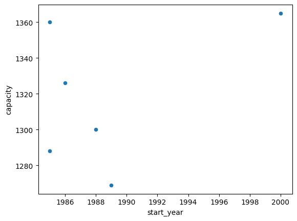

df.capacity.plot.barh(color="orange")
import matplotlib.pyplot as plt

plt.xlabel("Capacity (MW)")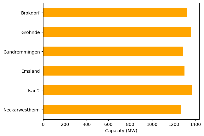

Time Indexes¶

Indexes are very powerful. They are a big part of why Pandas is so useful. There are different indices for different types of data. Time Indexes are especially great when handling time-dependent data.

time = pd.date_range(start="2021-01-01", end="2023-01-01", freq="D")
time.dayofyear

Index([  1,   2,   3,   4,   5,   6,   7,   8,   9,  10,
       ...
       357, 358, 359, 360, 361, 362, 363, 364, 365,   1],
      dtype='int32', length=731)

values = np.sin(2 * np.pi * time.dayofyear / 365)
values

Index([ 0.017213356155834685,   0.03442161162274574,  0.051619667223253764,
         0.06880242680231986,   0.08596479873744647,   0.10310169744743485,
          0.1202080448993527,   0.13727877211326478,   0.15430882066428117,
          0.1712931441814776,
       ...
        -0.13727877211326517,  -0.12020804489935275,  -0.10310169744743544,
         -0.0859647987374467,  -0.06880242680232064,  -0.05161966722325418,
       -0.034421611622745804,  -0.01721335615583528, 6.432490598706546e-16,
        0.017213356155834685],
      dtype='float64', length=731)

values = np.sin(2 * np.pi * time.dayofyear / 365)
ts = pd.Series(values, index=time)
ts

2021-01-01    1.721336e-02
2021-01-02    3.442161e-02
2021-01-03    5.161967e-02
2021-01-04    6.880243e-02
2021-01-05    8.596480e-02
                  ...     
2022-12-28   -5.161967e-02
2022-12-29   -3.442161e-02
2022-12-30   -1.721336e-02
2022-12-31    6.432491e-16
2023-01-01    1.721336e-02
Freq: D, Length: 731, dtype: float64

ts.plot()

<Axes: >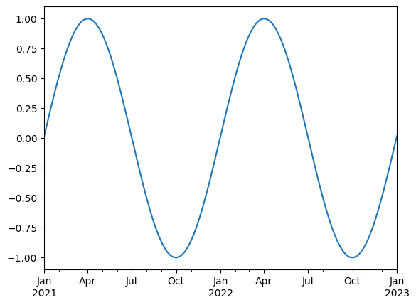

We can use Python’s slicing notation inside .loc to select a date range.

ts.loc["2021-01-01":"2021-07-01"].plot()

<Axes: >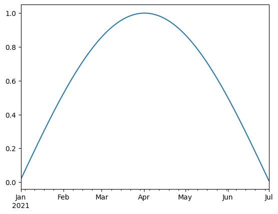

ts.loc["2021-05"].plot()

<Axes: >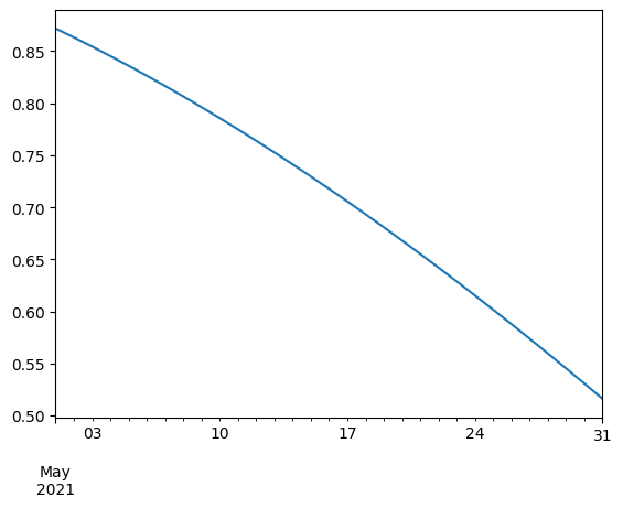

The pd.TimeIndex object has lots of useful attributes

ts.index.month

Index([ 1,  1,  1,  1,  1,  1,  1,  1,  1,  1,
       ...
       12, 12, 12, 12, 12, 12, 12, 12, 12,  1],
      dtype='int32', length=731)

ts.index.weekday

Index([4, 5, 6, 0, 1, 2, 3, 4, 5, 6,
       ...
       4, 5, 6, 0, 1, 2, 3, 4, 5, 6],
      dtype='int32', length=731)

Another common operation is to change the resolution of a dataset by resampling in time. Pandas exposes this through the .resample() function. The resample periods are specified using pandas offset index syntax.

Below, we resample the dataset by taking the mean over each month.

ts.resample("12h").mean().interpolate()

2021-01-01 00:00:00    1.721336e-02
2021-01-01 12:00:00    2.581748e-02
2021-01-02 00:00:00    3.442161e-02
2021-01-02 12:00:00    4.302064e-02
2021-01-03 00:00:00    5.161967e-02
                           ...     
2022-12-30 00:00:00   -1.721336e-02
2022-12-30 12:00:00   -8.606678e-03
2022-12-31 00:00:00    6.432491e-16
2022-12-31 12:00:00    8.606678e-03
2023-01-01 00:00:00    1.721336e-02
Freq: 12h, Length: 1461, dtype: float64

ts.resample("ME").mean().plot()

<Axes: >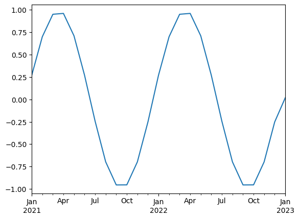

Reading and Writing Files¶

To read data into pandas, we can use for instance the pd.read_csv() function. This function is quite powerful and complex with many different settings. You can use it to extract data from almost any text file.

The pd.read_csv() function can take a path to a local file as an input, or even a hyperlink to an online text file.

Let’s import a slightly larger dataset about the power plant fleet in Europe_

fn = "https://raw.githubusercontent.com/PyPSA/powerplantmatching/master/powerplants.csv"
# fn = "powerplants(4).csv"

df = pd.read_csv(fn, index_col=0)

df = pd.read_csv(fn, index_col=0)
df.iloc[:5, :10]

df.info()

<class 'pandas.core.frame.DataFrame'>
Index: 158548 entries, 0 to 159062
Data columns (total 18 columns):
 #   Column               Non-Null Count   Dtype  
---  ------               --------------   -----  
 0   Name                 158548 non-null  object 
 1   Fueltype             158548 non-null  object 
 2   Technology           106116 non-null  object 
 3   Set                  158169 non-null  object 
 4   Country              158548 non-null  object 
 5   Capacity             158514 non-null  float64
 6   Efficiency           510 non-null     float64
 7   DateIn               153762 non-null  float64
 8   DateRetrofit         2553 non-null    float64
 9   DateOut              4720 non-null    float64
 10  lat                  158548 non-null  float64
 11  lon                  158548 non-null  float64
 12  Duration             1853 non-null    float64
 13  Volume_Mm3           1762 non-null    float64
 14  DamHeight_m          2010 non-null    float64
 15  StorageCapacity_MWh  2402 non-null    float64
 16  EIC                  158548 non-null  object 
 17  projectID            158548 non-null  object 
dtypes: float64(11), object(7)
memory usage: 23.0+ MB

df.describe()

Sometimes, we also want to store a DataFrame for later use. There are many different file formats tabular data can be stored in, including HTML, JSON, Excel, Parquet, Feather, etc. Here, let’s say we want to store the DataFrame as CSV (comma-separated values) file under the name “tmp.csv”.

df.to_csv("tmp.csv")

df

Grouping and Aggregation¶

Both Series and DataFrame objects have a groupby method, which allows you to group and aggregate the data based on the values of one or more columns.

It accepts a variety of arguments, but the simplest way to think about it is that you pass another series, whose unique values are used to split the original object into different groups.

Here’s an example which retrieves the total generation capacity per country.

grouped = df.groupby("Country").Capacity.sum()
grouped.sort_values(ascending=False).head(10)

Country
Germany           326960.298047
United Kingdom    161132.840000
France            154211.172001
Spain             139610.514800
Italy             104771.038000
Poland             60847.866738
Ukraine            57548.700000
Sweden             51995.322323
Netherlands        42405.100000
Norway             40624.110000
Name: Capacity, dtype: float64

Such chaining of multiple operations is very common with pandas.

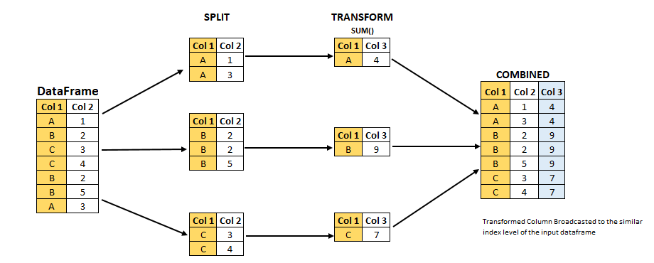
Let’s break apart this operation a bit. The workflow with groupby can be divided into three general steps:

Split: Partition the data into different groups based on some criterion.
Apply: Do some calculation (e.g. aggregation or transformation) within each group.
Combine: Put the results back together into a single object.

Grouping is not only possible on a single columns, but also on multiple columns. For instance, we might want to group the capacities by country and fuel type. To achieve this, we pass a list of functions to the groupby functions.

capacities = df.groupby(["Country", "Fueltype"]).Capacity.sum()
capacities

Country         Fueltype     
Albania         Hydro             2079.366
                Solar              394.500
                Wind               234.000
Austria         Battery             40.320
                Hard Coal         1471.000
                                   ...    
United Kingdom  Other               35.000
                Solar            12089.700
                Solid Biomass     4154.200
                Waste             1948.150
                Wind             37802.300
Name: Capacity, Length: 327, dtype: float64

By grouping by multiple attributes, our index becomes a pd.MultiIndex (a hierarchical index with multiple levels.

capacities.index[:5]

MultiIndex([('Albania',     'Hydro'),
            ('Albania',     'Solar'),
            ('Albania',      'Wind'),
            ('Austria',   'Battery'),
            ('Austria', 'Hard Coal')],
           names=['Country', 'Fueltype'])

type(capacities.index)

pandas.core.indexes.multi.MultiIndex

df.nsmallest(10, "Capacity")

We can use the .unstack function to reshape the multi-indexed pd.Series into a pd.DataFrame which has the second index level as columns.

capacities.unstack().fillna(0.0).T.round(1)

In summary, the typical workflow with pandas consists of reading data from files, inspecting and cleaning the data, performing analysis through transformation and aggregation, visualizing the results, and storing the processed data for later use.

Exercises¶

Power Plants Data¶

In this exercise, we will use the powerplants.csv dataset from the powerplantmatching project. This dataset contains information about various power plants, including their names, countries, fuel types, capacities, and more.

URL: https://raw.githubusercontent.com/PyPSA/powerplantmatching/master/powerplants.csv

Task 1: Load the dataset into a pandas DataFrame.

Task 2: Run the function .describe() on the DataFrame.

Task 3: Provide a list of unique fuel types and technologies included in the dataset.

Task 4: Filter the dataset by power plants with the fuel type “Hard Coal”.

Task 5: Identify the 5 largest coal power plants. In which countries are they located? When were they built?

Task 6: Identify the power plant with the longest name.

Task 7: Identify the 10 northernmost powerplants. What type of power plants are they?

Task 8: What is the average start year of each fuel type? Sort the fuel types by their average start year in ascending order and round to the nearest integer.

Wind and Solar Capacity Factors¶

In this exercise, we will work with a time series dataset containing hourly wind and solar capacity factors for Ireland, taken from model.energy.

Task 1: Use pd.read_csv to load the dataset from the following URL into a pandas DataFrame. Ensure that the time stamps are treated as pd.DatetimeIndex.

Task 2: Calculate the mean capacity factor for wind and solar over the entire time period.

Task 3: Calculate the correlation between wind and solar capacity factors.

Task 4: Plot the wind and solar capacity factors for the month of May.

Task 5: Plot the weekly average capacity factors for wind and solar over the entire time period.

Task 6: Go to model.energy and retrieve the time series for another region of your choice. Recreate the analysis above and compare the results.

The Series¶

The DataFrame¶

Cleaning Data¶

Combining Datasets¶

Sorting & Filtering Data¶

Applying Functions¶

Plotting¶

Time Indexes¶

Reading and Writing Files¶

Grouping and Aggregation¶

Exercises¶

Power Plants Data¶

Wind and Solar Capacity Factors¶

The `Series`¶

The `DataFrame`¶