YouTube Video
Video not loading? Click here.
This workshop introduces you to interactive visualisation using the plotly library and the Streamlit framework for dashboards.
import pypsa
import atlite
import pandas as pd
import geopandas as gpdNotebook Cell
from urllib.request import urlretrieve
from os.path import basename

urls = [
    "https://tubcloud.tu-berlin.de/s/2oogpgBfM5n4ssZ/download/PORTUGAL-2013-01-era5.nc",
]
for url in urls:
    urlretrieve(url, basename(url))
Load Example Data
First, let’s load a few example datasets you know from previous tutorials.
A PyPSA network:
n = pypsa.Network(
    "https://tubcloud.tu-berlin.de/s/kpWaraGc9LeaxLK/download/network-cem.nc"
)
INFO:pypsa.network.io:Retrieving network data from https://tubcloud.tu-berlin.de/s/kpWaraGc9LeaxLK/download/network-cem.nc.
/home/runner/work/data-science-for-esm/data-science-for-esm/.venv/lib/python3.13/site-packages/xarray/backends/plugins.py:109: RuntimeWarning: Engine 'cfgrib' loading failed:
Cannot find the ecCodes library
  external_backend_entrypoints = backends_dict_from_pkg(entrypoints_unique)
WARNING:pypsa.network.io:Importing network from PyPSA version v1.0.3 while current version is v1.1.2. Read the release notes at `https://go.pypsa.org/release-notes` to prepare your network for import.
INFO:pypsa.network.io:New version 1.2.1 available! (Current: 1.1.2)
INFO:pypsa.network.io:Imported network 'Unnamed Network' has buses, carriers, generators, global_constraints, loads, storage_units, sub_networks
n.optimize();Output
INFO:linopy.model: Solve problem using Highs solver
INFO:linopy.io:Writing objective.
Writing constraints.: 0%| | 0/13 [00:00<?, ?it/s]Writing constraints.: 85%|████████▍ | 11/13 [00:00<00:00, 101.82it/s]Writing constraints.: 100%|██████████| 13/13 [00:00<00:00, 95.42it/s]
Writing continuous variables.: 0%| | 0/6 [00:00<?, ?it/s]Writing continuous variables.: 100%|██████████| 6/6 [00:00<00:00, 212.12it/s]
INFO:linopy.io: Writing time: 0.24s
Running HiGHS 1.14.0 (git hash: 7df0786): Copyright (c) 2026 under MIT licence terms
LP linopy-problem-crfrl6oa has 50377 rows; 21906 cols; 101886 nonzeros
Coefficient ranges:
  Matrix  [1e-04, 3e+02]
  Cost    [4e-02, 5e+05]
  Bound   [0e+00, 0e+00]
  RHS     [3e+04, 8e+04]
Presolving model
25230 rows, 18665 cols, 69120 nonzeros 0s
Dependent equations search running on 6570 equations with time limit of 1000.00s
Dependent equations search removed 0 rows and 0 nonzeros in 0.00s (limit = 1000.00s)
25230 rows, 18665 cols, 69120 nonzeros 0s
Presolve reductions: rows 25230(-25147); columns 18665(-3241); nonzeros 69120(-32766)
Solving the presolved LP
Using dual simplex solver
  Iteration        Objective     Infeasibilities num(sum)
          0     0.0000000000e+00 Pr: 2190(1.54362e+09) 0.1s
11919 1.8950944583e+10 Pr: 4368(1.08885e+14) 5.1s
18985 5.6631557832e+10 Pr: 6106(5.39821e+11); Du: 0(1.91928e-18) 10.2s
INFO:linopy.constants: Optimization successful:
Status: ok
Termination condition: optimal
Solution: 21906 primals, 50377 duals
Objective: 7.00e+10
Solver model: available
Solver message: Optimal
INFO:pypsa.optimization.optimize:The shadow-prices of the constraints Generator-ext-p-lower, Generator-ext-p-upper, StorageUnit-ext-p_dispatch-lower, StorageUnit-ext-p_dispatch-upper, StorageUnit-ext-p_store-lower, StorageUnit-ext-p_store-upper, StorageUnit-ext-state_of_charge-lower, StorageUnit-ext-state_of_charge-upper, StorageUnit-energy_balance were not assigned to the network.
      23889     6.9991508992e+10 Pr: 0(0); Du: 0(1.74222e-13) 12.3s

Performed postsolve
Solving the original LP from the solution after postsolve

Model name          : linopy-problem-crfrl6oa
Model status        : Optimal
Simplex   iterations: 23889
Objective value     :  6.9991508992e+10
P-D objective error :  2.0710868815e-15
HiGHS run time      :         12.34
Wind, solar and demand time series:
url = (
    "https://tubcloud.tu-berlin.de/s/nwCrNLrtL6LAN3W/download/time-series-lecture-2.csv"
)
ts = pd.read_csv(url, index_col=0, parse_dates=True)
Power plants in Europe
url = (
    "https://raw.githubusercontent.com/PyPSA/powerplantmatching/v0.7.1/powerplants.csv"
)
ppl = pd.read_csv(url, index_col=0).query("Fueltype not in ['Wind', 'Solar']")
geometry = gpd.points_from_xy(ppl["lon"], ppl["lat"])ppl = gpd.GeoDataFrame(ppl, geometry=geometry, crs=4326)NUTS2 regions:
url = "https://tubcloud.tu-berlin.de/s/RHZJrN8Dnfn26nr/download/NUTS_RG_10M_2021_4326.geojson"
nuts = gpd.read_file(url)
nuts = nuts.set_index("id").query("LEVL_CODE == 2")
An atlite cutout:
cutout = atlite.Cutout("PORTUGAL-2013-01-era5.nc")Limitations of Static Plots
You will agree that using matplotlib for static plotting is great for reports, but that it’s lacking some features for interactive visualisation.
ts["onwind [pu]"].plot(figsize=(10, 2))<Axes: >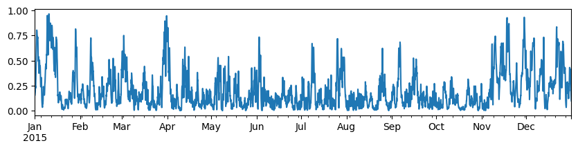
Interactive Plots with plotly
Specifically, we are going to use plotly.express, which is a high-level interface for plotly, to create interactive plots with just a few lines of code.
The
plotly.expressmodule (usually imported as px) contains functions that can create entire figures at once. Plotly Express is a built-in part of theplotlylibrary, and is the recommended starting point for creating most common figures. Every Plotly Express function uses graph objects internally and returns a plotly.graph_objects.Figure instance. Throughout the plotly documentation, you will find the Plotly Express way of building figures at the top of any applicable page, followed by a section on how to use graph objects to build similar figures. Any figure created in a single function call with Plotly Express could be created using graph objects alone, but with between 5 and 100 times more code.
import plotly.io as pio
import plotly.express as px
import plotly.offline as pyLet’s create a few plots!
Onshore wind capacity factor time series:
px.line(ts["onwind [pu]"])Load time series in February:
px.line(ts.loc["2015-02", "load [GW]"])Scatter plot on map of hard coal power plants in Europe:
df = ppl.query("Fueltype == 'Hard Coal'")px.scatter_mapbox(
df, lat="lat", lon="lon", mapbox_style="carto-positron", zoom=2, height=600
)/tmp/ipykernel_3161/2495599162.py:1: DeprecationWarning: *scatter_mapbox* is deprecated! Use *scatter_map* instead. Learn more at: https://plotly.com/python/mapbox-to-maplibre/
px.scatter_mapbox(
px.scatter_mapbox(
    df,
    lat="lat",
    lon="lon",
    mapbox_style="carto-positron",
    color="DateIn",
    size="Capacity",
    zoom=2,
    height=600,
)
/tmp/ipykernel_3161/3752641430.py:1: DeprecationWarning: *scatter_mapbox* is deprecated! Use *scatter_map* instead. Learn more at: https://plotly.com/python/mapbox-to-maplibre/
px.scatter_mapbox(
Choropleth map of NUTS2 regions coloured by country:
px.choropleth_mapbox(
    nuts,
    geojson=nuts.geometry,
    locations=nuts.index,
    mapbox_style="carto-positron",
    zoom=2,
    height=600,
    color="CNTR_CODE",
    center={"lat": 48, "lon": 12},
)
/tmp/ipykernel_3161/2861405607.py:1: DeprecationWarning: *choropleth_mapbox* is deprecated! Use *choropleth_map* instead. Learn more at: https://plotly.com/python/mapbox-to-maplibre/
px.choropleth_mapbox(
In plotly, hovering information can also be displayed well.
dispatch = (
    pd.concat([n.generators_t.p, n.storage_units_t.p], axis=1).loc["2015-02"].div(1e3)
)
df = dispatch.where(dispatch > 0, 0).stack().reset_index().rename(columns={0: "GW"})df.head(5)fig = px.area(df, x="snapshot", color="name", y="GW", line_group="name")
fig.update_traces(line=dict(width=0))
figInteractive Dashboards
There are many different options for building interactive dashboards (e.g., Dash, Streamlit, Panel). Some are brand new, some have been around for a few years. Here, we are going to work with Streamlit as one example, since it is relatively easy to get started with and produce first results quickly. However, compared to other dashboarding frameworks, it has some limitations in terms of layout and interactivity.
In this tutorial, we look at streamlit because it is the easiest to get to results quickly. However, compared to other dashboarding libraries, it has more limited configuration options.
Documentation for this package can be found here: https://
Streamlit can be installed (e.g. with minimum version 1.18), for example, with conda or pip:
conda install -c conda-forge streamlit'>=1.18'or
pip install streamlit">=1.18'The rest of the tutorial is contained in a separate repository on Github with instructions how to install, run and deploy it:
https://
You can see a live demo of the final product here: