YouTube Video
Video not loading? Click here.

Linopy is an open-source framework for formulating, solving, and analyzing optimization problems with Python.
With Linopy, you can create optimization models within Python that consist of decision variables, constraints, and optimization objectives. You can then solve these instances using a variety of commercial and open-source solvers (specialised software).
Linopy supports a wide range of problem types, including:
Linear programming
Integer programming
Mixed-integer programming
Quadratic programming
Solve a Basic Model
In this example, we explain the basic functions of the linopy Model class. First, we are setting up a very simple linear optimization model, given by
Minimize:
subject to:
Initializing a Model
The Model class in Linopy is a fundamental part of the library. It serves as a container for all the relevant data associated with a linear optimization problem. This includes variables, constraints, and the objective function.
import linopy

m = linopy.Model()
This creates a new Model object, which you can then use to define your optimization problem.
Adding decision variables
Variables are the unknowns of an optimisation problems and are intended to be given values by solving an optimisation problem. A variable can always be assigned with a lower and an upper bound. In our case, both x and y have a lower bound of zero (default is unbouded). In linopy, you can add variables to a Model using the add_variables() method:
x = m.add_variables(lower=0, name="x")
y = m.add_variables(lower=0, name="y");
x and y are linopy variables of the class linopy.Variable. Each of them contain all relevant information that define it. The name parameter is optional but can be useful for referencing the variables later.
xVariable
--------
x ∈ [0, inf]m.variableslinopy.model.Variables
----------------------
* x
* ym.variables["x"]Variable
--------
x ∈ [0, inf]Adding Constraints
Constraints are equality or inequality expressions that define the feasible space of the decision variables. They consist of the left hand side (LHS) and the right hand side (RHS). The first constraint that we want to write down is which we write out exactly in the mathematical way:
3 * x + 7 * y >= 10Constraint (unassigned)
-----------------------
+3 x + 7 y ≥ 10.0Note, we can also mix the constant and the variable expression, like this
3 * x + 7 * y - 10 >= 0Constraint (unassigned)
-----------------------
+3 x + 7 y ≥ 10.0… and linopy will automatically take over the separation of variables expression on the LHS, and constant values on the RHS.
The constraint is currently not assigned to the model. We assign it by calling the add_constraints() function:
m.add_constraints(3 * x + 7 * y >= 10)
m.add_constraints(5 * x + 2 * y >= 3);m.constraintslinopy.model.Constraints
------------------------
* con0
* con1m.constraints["con0"]Constraint `con0`
-----------------
+3 x + 7 y ≥ 10.0Adding the Objective
The objective function defines what you want to optimize. It is a function of variables that a solver attempts to maximize or minimize. You can set the objective function of a linopy.Model using the add_objective() method. For our example that would be
m.add_objective(x + 2 * y, sense="min")m.objectiveObjective:
----------
LinearExpression: +1 x + 2 y
Sense: min
Value: NoneNote, we can either minimize or maximize in linopy. Per default, linopy applies sense='min' so it is not necessary to explicitly define the optimization sense. In summary:
mLinopy LP model
===============
Variables:
----------
* x
* y
Constraints:
------------
* con0
* con1
Status:
-------
initializedSolving the Model
Once you’ve defined your linopy.Model with variables, constraints, and an objective function, you can solve it using the solve method:
m.solve()Running HiGHS 1.14.0 (git hash: 7df0786): Copyright (c) 2026 under MIT licence terms
LP linopy-problem-y5y74uof has 2 rows; 2 cols; 4 nonzeros
Coefficient ranges:
Matrix [2e+00, 7e+00]
Cost [1e+00, 2e+00]
Bound [0e+00, 0e+00]
RHS [3e+00, 1e+01]
Presolving model
2 rows, 2 cols, 4 nonzeros 0s
2 rows, 2 cols, 4 nonzeros 0s
Presolve reductions: rows 2(-0); columns 2(-0); nonzeros 4(-0) - Not reduced
Problem not reduced by presolve: solving the LP
Using dual simplex solver
Iteration Objective Infeasibilities num(sum)
0 0.0000000000e+00 Pr: 2(13) 0.0s
2 2.8620689655e+00 Pr: 0(0) 0.0s
Model name : linopy-problem-y5y74uof
Model status : Optimal
Simplex iterations: 2
Objective value : 2.8620689655e+00
P-D objective error : 0.0000000000e+00
HiGHS run time : 0.00
('ok', 'optimal')Solvers are needed to compute solutions to the optimization models. There exists a large variety of solvers. In many cases, they specialise in certain problem types or solving algorithms, e.g. linear or nonlinear problems.
commercial examples: Gurobi, COPT CPLEX, FICO Xpress
The open-source solvers are sufficient to handle meaningful linopy models with hundreds to several thousand variables and constraints. However, as applications get large or more complex, there may be a need to turn to a commercial solvers (which often provide free academic licenses).
For this course, we use HiGHS, which is already in the course environment esm-ss-26.
Retrieving optimisation results
The solution of the linear problem is assigned to the variables under solution in form of a xarray.Dataset.
x.solutiony.solutionWe can also read out the objective value:
m.objective.value2.8620689655172415And the dual values (or shadow prices) of the model’s constraints:
m.dual["con0"]Well done! You solved your first linopy model!
Use Coordinates
Now, the real power of the package comes into play!
Linopy is structured around the concept that variables, and therefore expressions and constraints, have coordinates. That is, a Variable object actually contains multiple variables across dimensions, just as we know it from a numpy array or a pandas.DataFrame.
Suppose the two variables x and y are now functions of time t and we would modify the problem according to:
In order to formulate the new problem with linopy, we start again by initializing a model.
m = linopy.Model()Again, we define x and y using the add_variables() function, but now we are adding a coords argument. This automatically creates optimization variables for all coordinates, in this case time-steps t.
import pandas as pd

time = pd.Index(range(10), name="time")

x = m.add_variables(
    lower=0,
    coords=[time],
    name="x",
)
y = m.add_variables(lower=0, coords=[time], name="y")xVariable (time: 10)
-------------------
[0]: x[0] ∈ [0, inf]
[1]: x[1] ∈ [0, inf]
[2]: x[2] ∈ [0, inf]
[3]: x[3] ∈ [0, inf]
[4]: x[4] ∈ [0, inf]
[5]: x[5] ∈ [0, inf]
[6]: x[6] ∈ [0, inf]
[7]: x[7] ∈ [0, inf]
[8]: x[8] ∈ [0, inf]
[9]: x[9] ∈ [0, inf]Following the previous example, we write the constraints out using the syntax from above, while multiplying the RHS with t. Note that the coordinates from the LHS and the RSH have to match.
factor = pd.Series(time, index=time)

3 * x + 7 * y >= 10 * factor
Constraint (unassigned) [time: 10]:
-----------------------------------
[0]: +3 x[0] + 7 y[0] ≥ -0.0
[1]: +3 x[1] + 7 y[1] ≥ 10.0
[2]: +3 x[2] + 7 y[2] ≥ 20.0
[3]: +3 x[3] + 7 y[3] ≥ 30.0
[4]: +3 x[4] + 7 y[4] ≥ 40.0
[5]: +3 x[5] + 7 y[5] ≥ 50.0
[6]: +3 x[6] + 7 y[6] ≥ 60.0
[7]: +3 x[7] + 7 y[7] ≥ 70.0
[8]: +3 x[8] + 7 y[8] ≥ 80.0
[9]: +3 x[9] + 7 y[9] ≥ 90.0It always helps to write out the constraints before adding them to the model. Since they look good, let’s assign them.
con1 = m.add_constraints(3 * x + 7 * y >= 10 * factor, name="con1")
con2 = m.add_constraints(5 * x + 2 * y >= 3 * factor, name="con2")
m
Linopy LP model
===============
Variables:
----------
* x (time)
* y (time)
Constraints:
------------
* con1 (time)
* con2 (time)
Status:
-------
initializedNow, when it comes to the objective, we use the sum function of linopy.LinearExpression. This stacks all terms all terms of the time dimension and writes them into one big expression.
obj = (x + 2 * y).sum()objLinearExpression
----------------
+1 x[0] + 2 y[0] + 1 x[1] ... +2 y[8] + 1 x[9] + 2 y[9]m.add_objective(obj, overwrite=True)Then, we can solve:
m.solve()Running HiGHS 1.14.0 (git hash: 7df0786): Copyright (c) 2026 under MIT licence terms
LP linopy-problem-880hwl1g has 20 rows; 20 cols; 40 nonzeros
Coefficient ranges:
Matrix [2e+00, 7e+00]
Cost [1e+00, 2e+00]
Bound [0e+00, 0e+00]
RHS [3e+00, 9e+01]
Presolving model
18 rows, 18 cols, 36 nonzeros 0s
18 rows, 18 cols, 36 nonzeros 0s
Presolve reductions: rows 18(-2); columns 18(-2); nonzeros 36(-4)
Solving the presolved LP
Using dual simplex solver
Iteration Objective Infeasibilities num(sum)
0 0.0000000000e+00 Pr: 18(585) 0.0s
18 1.2879310345e+02 Pr: 0(0) 0.0s
Performed postsolve
Solving the original LP from the solution after postsolve
Model name : linopy-problem-880hwl1g
Model status : Optimal
Simplex iterations: 18
Objective value : 1.2879310345e+02
P-D objective error : 0.0000000000e+00
HiGHS run time : 0.00
('ok', 'optimal')In order to inspect the solution. You can go via the variables, i.e. y.solution or via the solution aggregator of the model, which combines the solution of all variables.
m.solution.to_dataframe()Sometimes it can be helpful to plot the solution:
m.solution.to_dataframe().plot(grid=True, ylabel="Optimal Value");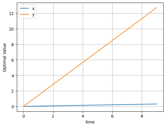
Alright! Now you learned how to set up linopy variables and expressions with coordinates. For more advanced linopy operations you can check out the User Guide.
Electricity Market Examples
Single bidding zone, single period
We want to minimise operational cost of an example electricity system representing South Africa subject to generator limits and meeting the load:
such that
We are given the following information on the South African electricity system:
Marginal costs in EUR/MWh
marginal_costs = pd.Series([0, 30, 60, 80], index=["Wind", "Coal", "Gas", "Oil"])
marginal_costs
Wind 0
Coal 30
Gas 60
Oil 80
dtype: int64Power plant capacities in MW
capacities = pd.Series([3000, 35000, 8000, 2000], index=["Wind", "Coal", "Gas", "Oil"])
capacities
Wind 3000
Coal 35000
Gas 8000
Oil 2000
dtype: int64Inelastic demand in MW
load = 42000We now start building the model
m = linopy.Model()g = m.add_variables(lower=0, upper=capacities, coords=[capacities.index], name="g")
gVariable (dim_0: 4)
-------------------
[Wind]: g[Wind] ∈ [0, 3000]
[Coal]: g[Coal] ∈ [0, 3.5e+04]
[Gas]: g[Gas] ∈ [0, 8000]
[Oil]: g[Oil] ∈ [0, 2000]And and the objective to minimize total operational costs:
m.add_objective(marginal_costs.values * g, sense="min")
m.objective
Objective:
----------
LinearExpression: +0 g[Wind] + 30 g[Coal] + 60 g[Gas] + 80 g[Oil]
Sense: min
Value: NoneWhich is subject to:
m.add_constraints(g.sum() == load, name="energy_balance")Constraint `energy_balance`
---------------------------
+1 g[Wind] + 1 g[Coal] + 1 g[Gas] + 1 g[Oil] = 42000.0Then, we can solve the model:
m.solve()Running HiGHS 1.14.0 (git hash: 7df0786): Copyright (c) 2026 under MIT licence terms
LP linopy-problem-tfuxd1xk has 1 row; 4 cols; 4 nonzeros
Coefficient ranges:
Matrix [1e+00, 1e+00]
Cost [3e+01, 8e+01]
Bound [2e+03, 4e+04]
RHS [4e+04, 4e+04]
Presolving model
1 rows, 3 cols, 3 nonzeros 0s
0 rows, 0 cols, 0 nonzeros 0s
Presolve reductions: rows 0(-1); columns 0(-4); nonzeros 0(-4) - Reduced to empty
Performed postsolve
Solving the original LP from the solution after postsolve
Model name : linopy-problem-tfuxd1xk
Model status : Optimal
Objective value : 1.2900000000e+06
P-D objective error : 0.0000000000e+00
HiGHS run time : 0.00
('ok', 'optimal')This is the optimimal generator dispatch (MW)
m.solution.to_dataframe()And the market clearing price we can read from the shadow price of the energy balance constraint (i.e. the added cost of increasing electricity demand by one unit):
m.dual["energy_balance"]Two bidding zones with transmission
Let’s add a spatial dimension, such that the optimisation problem is expanded to
such that
In this example, we connect the previous South African electricity system with a hydro generation unit in Mozambique through a single transmission line. Note that because a single transmission line will not result in any cycles, we can neglect KVL in this case.
We are given the following data (all in MW):
generators = ["Coal", "Wind", "Gas", "Oil", "Hydro"]
countries = ["South_Africa", "Mozambique"]
capacities = pd.DataFrame(
{
"Coal": [35000, 0],
"Wind": [3000, 0],
"Gas": [8000, 0],
"Oil": [2000, 0],
"Hydro": [0, 1200],
},
index=countries,
)
capacities.index.name = "countries"
capacities.columns.name = "generators"
capacities# variable costs in EUR/MWh
marginal_costs = pd.Series([30, 0, 60, 80, 0], index=generators)
marginal_costs.index.name = "generators"
marginal_costsgenerators
Coal 30
Wind 0
Gas 60
Oil 80
Hydro 0
dtype: int64load = pd.Series([42000, 650], index=countries)
load.index.name = "countries"
loadcountries
South_Africa 42000
Mozambique 650
dtype: int64transmission = 500Let’s start with a new model instance
m = linopy.Model()Now we create dispatch variables, as before, with the upper and lower bound for each countries and generators.
capacitiesg = m.add_variables(lower=0, upper=capacities, name="g")
gVariable (countries: 2, generators: 5)
--------------------------------------
[South_Africa, Coal]: g[South_Africa, Coal] ∈ [0, 3.5e+04]
[South_Africa, Wind]: g[South_Africa, Wind] ∈ [0, 3000]
[South_Africa, Gas]: g[South_Africa, Gas] ∈ [0, 8000]
[South_Africa, Oil]: g[South_Africa, Oil] ∈ [0, 2000]
[South_Africa, Hydro]: g[South_Africa, Hydro] ∈ [0, 0]
[Mozambique, Coal]: g[Mozambique, Coal] ∈ [0, 0]
[Mozambique, Wind]: g[Mozambique, Wind] ∈ [0, 0]
[Mozambique, Gas]: g[Mozambique, Gas] ∈ [0, 0]
[Mozambique, Oil]: g[Mozambique, Oil] ∈ [0, 0]
[Mozambique, Hydro]: g[Mozambique, Hydro] ∈ [0, 1200]We now define the line limit for the transmission line, assuming that power flowing from Mozambique to South Africa is positive.
The line limit equation can be defined as
f = m.add_variables(lower=-transmission, upper=transmission, name="flow_MZ_SA")
f
Variable
--------
flow_MZ_SA ∈ [-500, 500]The energy balance constraint is replaced by KCL, where we take into account local generation as well as incoming or outgoing flows. The KCL equation can be defined as:
We also need the incidence matrix of this network (here it’s very simple!) and assume some direction for the flow variable. Here, we picked the orientation from South Africa to Mozambique. This means that if the values for the flow variable are positive South Africa exports to Mozambique and vice versa if the variable takes negative values.
for country in countries:
    sign = -1 if country == "Mozambique" else 1  # minimal incidence matrix
    m.add_constraints(
        g.loc[country].sum() + sign * f == load[country],
        name=f"{country}_KCL",
)m.constraints["Mozambique_KCL"]Constraint `Mozambique_KCL`
---------------------------
+1 g[Mozambique, Coal] + 1 g[Mozambique, Wind] + 1 g[Mozambique, Gas] + 1 g[Mozambique, Oil] + 1 g[Mozambique, Hydro] - 1 flow_MZ_SA = 650.0The objective can be written as:
obj = (g * marginal_costs).sum()
obj
LinearExpression
----------------
+30 g[South_Africa, Coal] + 30 g[Mozambique, Coal] + 0 g[South_Africa, Wind] ... +80 g[Mozambique, Oil] + 0 g[South_Africa, Hydro] + 0 g[Mozambique, Hydro]m.add_objective(obj, sense="min")We now solve the model.
m.solve()Running HiGHS 1.14.0 (git hash: 7df0786): Copyright (c) 2026 under MIT licence terms
LP linopy-problem-p6j7bocp has 2 rows; 11 cols; 12 nonzeros
Coefficient ranges:
Matrix [1e+00, 1e+00]
Cost [3e+01, 8e+01]
Bound [5e+02, 4e+04]
RHS [6e+02, 4e+04]
Presolving model
1 rows, 4 cols, 4 nonzeros 0s
0 rows, 0 cols, 0 nonzeros 0s
Presolve reductions: rows 0(-2); columns 0(-11); nonzeros 0(-12) - Reduced to empty
Performed postsolve
Solving the original LP from the solution after postsolve
Model name : linopy-problem-p6j7bocp
Model status : Optimal
Objective value : 1.2600000000e+06
P-D objective error : 0.0000000000e+00
HiGHS run time : 0.00
('ok', 'optimal')Now, we print the optimization results
m.objective.value1260000.0g.solution.to_dataframe()m.constraints["South_Africa_KCL"].dualm.constraints["Mozambique_KCL"].dualSingle bidding zone with several periods
In this example, we consider multiple time periods (labelled [0,1,2,3]) to represent variable wind generation and changing load.
We are given the following data as before, just dropping Mozambique:
capacities = capacities.loc["South_Africa"]time_index = pd.Index([0, 1, 2, 3], name="time")
time_indexIndex([0, 1, 2, 3], dtype='int64', name='time')capacity_factors = pd.DataFrame(
{
"Coal": 4 * [1],
"Wind": [0.3, 0.6, 0.4, 0.5],
"Gas": 4 * [1],
"Oil": 4 * [1],
"Hydro": 4 * [1],
},
index=time_index,
columns=generators,
)
capacity_factors.index.name = "time"
capacity_factors.columns.name = "generators"
capacity_factorsload = pd.Series([42000, 43000, 45000, 46000], index=time_index)
load.index.name = "time"We now start building the model:
m = linopy.Model()Let’s define the dispatch variables g with the lower and upper bound:
g = m.add_variables(lower=0, upper=capacities * capacity_factors, name="g")
g
Variable (time: 4, generators: 5)
---------------------------------
[0, Coal]: g[0, Coal] ∈ [0, 3.5e+04]
[0, Wind]: g[0, Wind] ∈ [0, 900]
[0, Gas]: g[0, Gas] ∈ [0, 8000]
[0, Oil]: g[0, Oil] ∈ [0, 2000]
[0, Hydro]: g[0, Hydro] ∈ [0, 0]
[1, Coal]: g[1, Coal] ∈ [0, 3.5e+04]
[1, Wind]: g[1, Wind] ∈ [0, 1800]
...
[2, Oil]: g[2, Oil] ∈ [0, 2000]
[2, Hydro]: g[2, Hydro] ∈ [0, 0]
[3, Coal]: g[3, Coal] ∈ [0, 3.5e+04]
[3, Wind]: g[3, Wind] ∈ [0, 1500]
[3, Gas]: g[3, Gas] ∈ [0, 8000]
[3, Oil]: g[3, Oil] ∈ [0, 2000]
[3, Hydro]: g[3, Hydro] ∈ [0, 0]Then, we add the objective:
m.add_objective((g * marginal_costs).sum(), sense="min")
m.objective
Objective:
----------
LinearExpression: +30 g[0, Coal] + 30 g[1, Coal] + 30 g[2, Coal] ... +0 g[1, Hydro] + 0 g[2, Hydro] + 0 g[3, Hydro]
Sense: min
Value: NoneWhich is subject to:
m.add_constraints(
    g.sum("generators") == load,
    name="energy_balance",
)
Constraint `energy_balance` [time: 4]:
--------------------------------------
[0]: +1 g[0, Coal] + 1 g[0, Wind] + 1 g[0, Gas] + 1 g[0, Oil] + 1 g[0, Hydro] = 42000.0
[1]: +1 g[1, Coal] + 1 g[1, Wind] + 1 g[1, Gas] + 1 g[1, Oil] + 1 g[1, Hydro] = 43000.0
[2]: +1 g[2, Coal] + 1 g[2, Wind] + 1 g[2, Gas] + 1 g[2, Oil] + 1 g[2, Hydro] = 45000.0
[3]: +1 g[3, Coal] + 1 g[3, Wind] + 1 g[3, Gas] + 1 g[3, Oil] + 1 g[3, Hydro] = 46000.0We now solve the model:
m.solve()Running HiGHS 1.14.0 (git hash: 7df0786): Copyright (c) 2026 under MIT licence terms
LP linopy-problem-vjienj13 has 4 rows; 20 cols; 20 nonzeros
Coefficient ranges:
Matrix [1e+00, 1e+00]
Cost [3e+01, 8e+01]
Bound [9e+02, 4e+04]
RHS [4e+04, 5e+04]
Presolving model
4 rows, 12 cols, 12 nonzeros 0s
0 rows, 0 cols, 0 nonzeros 0s
Presolve reductions: rows 0(-4); columns 0(-20); nonzeros 0(-20) - Reduced to empty
Performed postsolve
Solving the original LP from the solution after postsolve
Model name : linopy-problem-vjienj13
Model status : Optimal
Objective value : 6.0820000000e+06
P-D objective error : 0.0000000000e+00
HiGHS run time : 0.00
('ok', 'optimal')We display the results. For ease of reading, we round the results to 2 decimals:
m.objective.value6082000.0g.solution.round(2).to_dataframe().squeeze().unstack()m.dual.to_dataframe()Single bidding zone with several periods and storage
Now, we want to expand the optimisation model with a storage unit to do price arbitrage to reduce oil consumption.
We have been given the following characteristics of the storage:
storage_energy = 6000  # MWh
storage_power = 1000  # MW
efficiency = 0.9  # discharge = charge
standing_loss = 0.00001 # per hourmLinopy LP model
===============
Variables:
----------
* g (time, generators)
Constraints:
------------
* energy_balance (time)
Status:
-------
okTo model a storage unit, we need three additional variables for the discharging and charging of the storage unit and for its state of charge (energy filling level). We can directly define the bounds of these variables in the variable definition:
battery_discharge = m.add_variables(
    lower=0, upper=storage_power, coords=[time_index], name="battery_discharge"
)
battery_charge = m.add_variables(
    lower=0, upper=storage_power, coords=[time_index], name="battery_charge"
)
battery_soc = m.add_variables(
    lower=0, upper=storage_energy, coords=[time_index], name="battery_soc"
)
Then, we implement the storage consistency equations,
For the initial period, we set the state of charge to zero.
m.add_constraints(battery_soc.loc[0] == 0, name="soc_initial")Constraint `soc_initial`
------------------------
+1 battery_soc[0] = -0.0m.add_constraints(
battery_soc.loc[1:]
== (1 - standing_loss) * battery_soc.shift(time=1).loc[1:]
+ efficiency * battery_charge.loc[1:]
- 1 / efficiency * battery_discharge.loc[1:],
name="soc_consistency",
)Constraint `soc_consistency` [time: 3]:
---------------------------------------
[1]: +1 battery_soc[1] - 1 battery_soc[0] - 0.9 battery_charge[1] + 1.111 battery_discharge[1] = -0.0
[2]: +1 battery_soc[2] - 1 battery_soc[1] - 0.9 battery_charge[2] + 1.111 battery_discharge[2] = -0.0
[3]: +1 battery_soc[3] - 1 battery_soc[2] - 0.9 battery_charge[3] + 1.111 battery_discharge[3] = -0.0And we also need to modify the energy balance to include the contributions of storage discharging and charging.
For that, we should first remove the existing energy balance constraint, which we seek to overwrite.
m.remove_constraints("energy_balance")m.add_constraints(
g.sum("generators") + battery_discharge - battery_charge == load,
name="energy_balance",
)Constraint `energy_balance` [time: 4]:
--------------------------------------
[0]: +1 g[0, Coal] + 1 g[0, Wind] + 1 g[0, Gas] ... +1 g[0, Hydro] + 1 battery_discharge[0] - 1 battery_charge[0] = 42000.0
[1]: +1 g[1, Coal] + 1 g[1, Wind] + 1 g[1, Gas] ... +1 g[1, Hydro] + 1 battery_discharge[1] - 1 battery_charge[1] = 43000.0
[2]: +1 g[2, Coal] + 1 g[2, Wind] + 1 g[2, Gas] ... +1 g[2, Hydro] + 1 battery_discharge[2] - 1 battery_charge[2] = 45000.0
[3]: +1 g[3, Coal] + 1 g[3, Wind] + 1 g[3, Gas] ... +1 g[3, Hydro] + 1 battery_discharge[3] - 1 battery_charge[3] = 46000.0We now solve the model:
m.solve()Running HiGHS 1.14.0 (git hash: 7df0786): Copyright (c) 2026 under MIT licence terms
LP linopy-problem-q_ksk4c5 has 8 rows; 32 cols; 41 nonzeros
Coefficient ranges:
Matrix [9e-01, 1e+00]
Cost [3e+01, 8e+01]
Bound [9e+02, 4e+04]
RHS [4e+04, 5e+04]
Presolving model
7 rows, 21 cols, 29 nonzeros 0s
Dependent equations search running on 4 equations with time limit of 1000.00s
Dependent equations search removed 0 rows and 0 nonzeros in 0.00s (limit = 1000.00s)
4 rows, 10 cols, 15 nonzeros 0s
Presolve reductions: rows 4(-4); columns 10(-22); nonzeros 15(-26)
Solving the presolved LP
Using dual simplex solver
Iteration Objective Infeasibilities num(sum)
0 5.3580000000e+06 Pr: 2(10300) 0.0s
7 6.0172006560e+06 Pr: 0(0) 0.0s
7 6.0172006560e+06 Pr: 0(0) 0.0s
Performed postsolve
Solving the original LP from the solution after postsolve
Model name : linopy-problem-q_ksk4c5
Model status : Optimal
Simplex iterations: 7
Objective value : 6.0172006560e+06
P-D objective error : 0.0000000000e+00
HiGHS run time : 0.00
('ok', 'optimal')We display the results:
m.objective.value6017200.65599352g.solution.to_dataframe().squeeze().unstack()battery_discharge.solution.to_dataframe()battery_charge.solution.to_dataframe()battery_soc.solution.to_dataframe()Exercise
Using the conversion efficiencies and specific emissions from the lecture slides, add a constraint that limits the total emissions in the four periods to 50% of the unconstrained optimal solution. How does the optimal objective value and the generator dispatch change?
Reimplement the storage consistency constraint such that the initial state of charge is not zero but corresponds to the state of charge in the final period of the optimisation horizon.
What parameters of the storage unit would have to be changed to reduce the objective? What’s the sensitivity?