PyPSA: Capacity Expansion - Data Science for Energy System Modelling

From electricity market modelling to capacity expansion planning¶

Review the problem formulation of the electricity market model. Below you can find an adapted version where the capacity limits have been promoted to decision variables with corresponding terms in the objective function and new constraints for their expansion limits (e.g. wind and solar potentials). This is known as capacity expansion problem.

\min_{g,e,f,G,E,F} \quad \sum_{i,s,t} w_t o_{s} g_{i,s,t} + \sum_{i,s} c_sG_{i,s} + c_{r,\text{dis/charge}}G_{i,r, \text{dis/charge}} + c_{r}E_{i,r} + c_\ell F_{\ell}

such that

\begin{align*} d_{i,t} &= \sum_s g_{i,s,t} - \sum_\ell K_{i\ell} f_{\ell,t} & \text{energy balance} \\ 0 &\leq g_{i,s,t} \leq \hat{g}_{i,s,t} G_{i,s} & \text{generator limits}\\ 0 & \leq g_{i,r,t,\text{dis/charge}} \leq G_{i,r,\text{dis/charge}}& \text{storage dis/charge limits} \\ 0 & \leq e_{i,r,t} \leq E_{r} & \text{storage energy limits} \\ e_{i,r,t} &= \eta^0_{i,r,t} e_{i,r,t-1} + \eta^1_{r}g_{i,r,t,\text{charge}} - \frac{1}{\eta^2_{r}} g_{i,r,t,\text{discharge}} & \text{storage consistency} \\ -F_\ell &\leq f_{\ell,t} \leq F_\ell & \text{line limits} \\ 0 &= \sum_\ell C_{\ell c} x_\ell f_{\ell,t} & \text{KVL} \\ \underline{G}_{i,s} & \leq G_{i,s} \leq \overline{G}_{i,s} & \text{generator capacity expansion limits} \\ \underline{G}_{i,r, \text{dis/charge}} & \leq G_{i,r, \text{dis/charge}} \leq \overline{G}_{i,r, \text{dis/charge}} & \text{storage power capacity expansion limits} \\ \underline{E}_{i,r} & \leq E_{i,r} \leq \overline{E}_{i,r} & \text{storage energy expansion limits} \\ \underline{F}_{\ell} & \leq F_{\ell} \leq \overline{F}_{\ell} & \text{line capacity expansion limits} \end{align*}

(1)

New decision variables for capacity expansion planning:

$G_{i,s}$ is the generator capacity at bus $i$ , technology $s$ ,
$F_{\ell}$ is the transmission capacity of line $\ell$ ,
$G_{i,r,\text{dis-/charge}}$ denotes the charge and discharge capacities of storage unit $r$ at bus $i$ ,
$E_{i,r}$ is the energy capacity of storage $r$ at bus $i$ and time step $t$ .

New parameters for capacity expansion planning:

$c_{\star}$ is the capital cost of technology $\star$ at bus $i$
$w_t$ is the weighting of time step $t$ (e.g. number of hours it represents)
$\underline{G}_\star, \underline{F}_\star, \underline{E}_\star$ are the minimum capacities per technology and location/connection.
$\underline{G}_\star, \underline{F}_\star, \underline{E}_\star$ are the maximum capacities per technology and location.

Note

If you have not yet set up Python on your computer, you can execute this tutorial in your browser via Google Colab. Download the .ipynb file using the download button on the top right corner and import it in Google Colab.

Then install the following packages by executing the following command in a Jupyter cell at the top of the notebook.

!pip install pypsa pandas matplotlib plotly"<6"

First things first! We need a few packages for this tutorial:

import pypsa
import pandas as pd
import matplotlib.pyplot as plt

import plotly.io as pio
import plotly.offline as py

pd.options.plotting.backend = "plotly"

Technology Data Inputs¶

We maintain a database (https://github.com/PyPSA/technology-data) which collects assumptions and projections for energy system technologies (such as costs, efficiencies, lifetimes, etc.) for given years, which we can load into a pandas.DataFrame. This requires some pre-processing to load (e.g. converting units, setting defaults, re-arranging dimensions):

year = 2030
url = f"https://raw.githubusercontent.com/PyPSA/technology-data/master/outputs/costs_{year}.csv"
costs = pd.read_csv(url, index_col=[0, 1])

costs.loc[costs.unit.str.contains("/kW"), "value"] *= 1e3
costs.unit = costs.unit.str.replace("/kW", "/MW")

defaults = {
    "FOM": 0,
    "VOM": 0,
    "efficiency": 1,
    "fuel": 0,
    "investment": 0,
    "lifetime": 25,
    "CO2 intensity": 0,
    "discount rate": 0.07,
}
costs = costs.value.unstack().fillna(defaults)

costs.at["OCGT", "fuel"] = costs.at["gas", "fuel"]
costs.at["CCGT", "fuel"] = costs.at["gas", "fuel"]
costs.at["OCGT", "CO2 intensity"] = costs.at["gas", "CO2 intensity"]
costs.at["CCGT", "CO2 intensity"] = costs.at["gas", "CO2 intensity"]

Let’s also import a small utility function that calculates the annuity to annualise investment costs. The formula is

a(r, n) = \frac{r}{1-(1+r)^{-n}}

(2)

where $r$ is the discount rate and $n$ is the lifetime. If $r=0$ , the annuity simplifies to $a(0,n) = \frac{1}{n}$ . If $n=\infty$ , the annuity simplifies to $a(r, \infty) = r$ .

from pypsa.common import annuity

annuity(0.07, 20)

0.09439292574325567

Based on this, we can calculate the short-term marginal generation costs (STMGC, €/MWh), named marginal_cost in PyPSA:

costs["marginal_cost"] = costs["VOM"] + costs["fuel"] / costs["efficiency"]

and the annualised investment costs (capital_cost in PyPSA terms, €/MW/a)

annuity_factor = annuity(costs["discount rate"], costs["lifetime"])

The FOM cost is expressed as a percentage of the overnight investment cost per year, and thus can be added to the annuity factor when calculating the annualised capital cost:

costs["capital_cost"] = (annuity_factor + costs["FOM"] / 100) * costs["investment"]

Loading time series data¶

We are also going to need some time series for wind, solar and load. For now, we are going to recycle the time series we used at the beginning of the course. They are given for Germany in the year 2015.

url = (
    "https://tubcloud.tu-berlin.de/s/pKttFadrbTKSJKF/download/time-series-lecture-2.csv"
)
ts = pd.read_csv(url, index_col=0, parse_dates=True)

ts.head(3)

Let’s convert the load time series from GW to MW, the base unit of PyPSA:

ts.load *= 1e3

We are also going to adapt the temporal resolution of the time series, e.g. sample only every other hour, to save some time:

resolution = 4
ts = ts.resample(f"{resolution}h").first()

Model Initialisation¶

In this section, we will build a replica of model.energy. This tool calculates the cost of meeting a constant electricity demand from a combination of wind power, solar power and storage for different regions of the world.

We deviate from model.energy by including offshore wind generation and electricity demand profiles rather than a constant electricity demand. Also, we are going to start with Germany only. You can adapt the code to other countries as an exercise.

For building the model, we start again by initialising an empty network.

n = pypsa.Network()

Then, we add a single bus...

n.add("Bus", "electricity", carrier="electricity")

...and tell the pypsa.Network object n that the snapshots of the model will be taken from the time series index ts.index.

n.snapshots = ts.index

n.snapshots[:12]

DatetimeIndex(['2015-01-01 00:00:00', '2015-01-01 04:00:00',
               '2015-01-01 08:00:00', '2015-01-01 12:00:00',
               '2015-01-01 16:00:00', '2015-01-01 20:00:00',
               '2015-01-02 00:00:00', '2015-01-02 04:00:00',
               '2015-01-02 08:00:00', '2015-01-02 12:00:00',
               '2015-01-02 16:00:00', '2015-01-02 20:00:00'],
              dtype='datetime64[ns]', name='snapshot', freq='4h')

The weighting of the snapshots (e.g. how many hours they represent, see $w_t$ in problem formulation above) can be set in n.snapshot_weightings.

n.snapshot_weightings.head(2)

n.snapshot_weightings.loc[:, :] = resolution

n.snapshot_weightings.head(2)

Adding Components¶

Then, we add all the technologies we are going to include as carriers.

carriers = [
    "onwind",
    "offwind",
    "solar",
    "OCGT",  # open cycle gas turbine
    "hydrogen storage underground",
    "battery storage",
    "electricity",
]

n.add(
    "Carrier",
    carriers,
    color=[
        "dodgerblue",
        "aquamarine",
        "gold",
        "indianred",
        "magenta",
        "yellowgreen",
        "black",
    ],
    co2_emissions=[
        costs.at[c, "CO2 intensity"] if c in costs.index else 0 for c in carriers
    ],
)

Next, we add the demand time series to the model.

n.add(
    "Load",
    "demand",
    bus="electricity",
    p_set=ts.load,
)

Let’s have a check whether the data was read-in correctly.

n.loads_t.p_set.plot(labels=dict(value="Load (MW)"))

We are going to add one dispatchable generation technology to the model. This is an open-cycle gas turbine (OCGT) with CO $_2$ emissions of 0.2 t/MWh $_{th}$ .

n.add(
    "Generator",
    "OCGT",
    bus="electricity",
    carrier="OCGT",
    capital_cost=costs.at["OCGT", "capital_cost"],
    marginal_cost=costs.at["OCGT", "marginal_cost"],
    efficiency=costs.at["OCGT", "efficiency"],
    p_nom_extendable=True,
)

Adding the variable renewable generators works almost identically, but we also need to supply the capacity factors to the model via the attribute p_max_pu.

for tech in ["onwind", "offwind", "solar"]:
    n.add(
        "Generator",
        tech,
        bus="electricity",
        carrier=tech,
        p_max_pu=ts[tech],
        capital_cost=costs.at[tech, "capital_cost"],
        marginal_cost=costs.at[tech, "marginal_cost"],
        efficiency=costs.at[tech, "efficiency"],
        p_nom_extendable=True,
    )

So let’s make sure the capacity factors are read-in correctly.

n.generators_t.p_max_pu.loc["2015-03"].plot(labels=dict(value="Capacity Factor [p.u.]"))

Model Run¶

Then, we can already solve the model for the first time. At this stage, the model does not have any storage or emission limits implemented. It’s going to look for the least-cost combination of variable renewables and the gas turbine to supply demand.

n.optimize(log_to_console=False)

INFO:linopy.model: Solve problem using Highs solver

INFO:linopy.model:Solver options:
 - log_to_console: False

INFO:linopy.io: Writing time: 0.08s

INFO:linopy.constants: Optimization successful: 
Status: ok
Termination condition: optimal
Solution: 8764 primals, 19714 duals
Objective: 3.16e+10
Solver model: available
Solver message: Optimal

INFO:pypsa.optimization.optimize:The shadow-prices of the constraints Generator-ext-p-lower, Generator-ext-p-upper were not assigned to the network.

('ok', 'optimal')

Model Evaluation¶

The total system cost in billion Euros per year:

n.objective / 1e9

31.62453194098724

The optimised capacities in GW:

n.generators.p_nom_opt.div(1e3)  # GW

name
OCGT       70.096357
onwind     -0.000000
offwind    49.326062
solar      85.967820
Name: p_nom_opt, dtype: float64

The energy balance by component in TWh:

n.statistics.energy_balance().sort_values().div(1e6)  # TWh

component  carrier  bus_carrier
Load       -        electricity   -478.925740
Generator  solar    electricity     92.766988
           offwind  electricity    150.379873
           OCGT     electricity    235.778879
dtype: float64

While we get the objective value through n.objective, in many cases we want to know how the costs are distributed across the technologies. We can use the statistics module for this:

(n.statistics.capex() + n.statistics.opex()).div(1e6)

component  carrier
Generator  OCGT       18596.014468
           offwind     8613.359135
           solar       4415.158338
dtype: float64

Possibly, we are also interested in the total emissions:

emissions = (
    n.generators_t.p
    / n.generators.efficiency
    * n.generators.carrier.map(n.carriers.co2_emissions)
)  # t/h

n.snapshot_weightings.generators @ emissions.sum(axis=1).div(1e6)  # Mt

np.float64(113.86394645337052)

The optimal dispatch time series can also be straightforwardly plotted, using the built-in plotting functionality of PyPSA.

n.statistics.energy_balance.iplot()

Adding Storage Units¶

Alright, but there are a few important components missing for a system with high shares of renewables? What about short-term storage options (e.g. batteries) and long-term storage options (e.g. hydrogen storage)? Let’s add them, too.

First, the battery storage. We are going to assume a fixed energy-to-power ratio of 4 hours, i.e. if fully charged, the battery can discharge at full capacity for 4 hours.

For the capital cost, we have to factor in both the capacity and energy cost of the storage. We are also going to enforce a cyclic state-of-charge condition, i.e. the state of charge at the beginning of the optimisation period must equal the final state of charge.

n.add(
    "StorageUnit",
    "battery storage",
    bus="electricity",
    carrier="battery storage",
    max_hours=4,
    capital_cost=costs.at["battery inverter", "capital_cost"]
    + 4 * costs.at["battery storage", "capital_cost"],
    efficiency_store=costs.at["battery inverter", "efficiency"],
    efficiency_dispatch=costs.at["battery inverter", "efficiency"],
    p_nom_extendable=True,
    cyclic_state_of_charge=True,
)

Second, the hydrogen storage. This one is composed of an electrolysis to convert electricity to hydrogen, a fuel cell (or hydrogen turbine) to re-convert hydrogen to electricity and underground storage (e.g. in salt caverns). We assume an energy-to-power ratio of 336 hours, such that this type of storage can be used for multi-week balancing.

capital_costs = (
    costs.at["electrolysis", "capital_cost"]
    + costs.at["fuel cell", "capital_cost"]
    + 336 * costs.at["hydrogen storage underground", "capital_cost"]
)

n.add(
    "StorageUnit",
    "hydrogen storage underground",
    bus="electricity",
    carrier="hydrogen storage underground",
    max_hours=336,
    capital_cost=capital_costs,
    efficiency_store=costs.at["electrolysis", "efficiency"],
    efficiency_dispatch=costs.at["fuel cell", "efficiency"],
    p_nom_extendable=True,
    cyclic_state_of_charge=True,
)

n.optimize(log_to_console=False)

INFO:linopy.model: Solve problem using Highs solver

INFO:linopy.model:Solver options:
 - log_to_console: False

INFO:linopy.io:Writing objective.

Writing constraints.:   0%|          | 0/12 [00:00<?, ?it/s]

Writing constraints.:  50%|█████     | 6/12 [00:00<00:00, 57.54it/s]

Writing constraints.: 100%|██████████| 12/12 [00:00<00:00, 47.66it/s]

Writing constraints.: 100%|██████████| 12/12 [00:00<00:00, 48.78it/s]

Writing continuous variables.:   0%|          | 0/6 [00:00<?, ?it/s]

Writing continuous variables.: 100%|██████████| 6/6 [00:00<00:00, 138.05it/s]


INFO:linopy.io: Writing time: 0.3s

INFO:linopy.constants: Optimization successful: 
Status: ok
Termination condition: optimal
Solution: 21906 primals, 50376 duals
Objective: 3.16e+10
Solver model: available
Solver message: Optimal

INFO:pypsa.optimization.optimize:The shadow-prices of the constraints Generator-ext-p-lower, Generator-ext-p-upper, StorageUnit-ext-p_dispatch-lower, StorageUnit-ext-p_dispatch-upper, StorageUnit-ext-p_store-lower, StorageUnit-ext-p_store-upper, StorageUnit-ext-state_of_charge-lower, StorageUnit-ext-state_of_charge-upper, StorageUnit-energy_balance were not assigned to the network.

('ok', 'optimal')

n.statistics.optimal_capacity().div(1e3)  # GW

component  carrier
Generator  OCGT       70.096357
           offwind    49.326062
           solar      85.967820
dtype: float64

Nothing! The objective value is the same, and no storage is built.

Adding emission limits¶

The gas power plant offers sufficient and cheap enough backup capacity to run in periods of low wind and solar generation. But what happens if this source of flexibility disappears. Let’s model a 100% renewable electricity system by adding a CO $_2$ emission limit as global constraint:

n.add(
    "GlobalConstraint",
    "CO2Limit",
    carrier_attribute="co2_emissions",
    sense="<=",
    constant=0,
)

When we run the model now...

n.optimize(log_to_console=False)

INFO:linopy.model: Solve problem using Highs solver

INFO:linopy.model:Solver options:
 - log_to_console: False

INFO:linopy.io:Writing objective.

Writing constraints.:   0%|          | 0/13 [00:00<?, ?it/s]

Writing constraints.:  62%|██████▏   | 8/13 [00:00<00:00, 79.61it/s]

Writing constraints.: 100%|██████████| 13/13 [00:00<00:00, 78.57it/s]

Writing continuous variables.:   0%|          | 0/6 [00:00<?, ?it/s]

Writing continuous variables.: 100%|██████████| 6/6 [00:00<00:00, 401.70it/s]


INFO:linopy.io: Writing time: 0.19s

INFO:linopy.constants: Optimization successful: 
Status: ok
Termination condition: optimal
Solution: 21906 primals, 50377 duals
Objective: 7.00e+10
Solver model: available
Solver message: Optimal

INFO:pypsa.optimization.optimize:The shadow-prices of the constraints Generator-ext-p-lower, Generator-ext-p-upper, StorageUnit-ext-p_dispatch-lower, StorageUnit-ext-p_dispatch-upper, StorageUnit-ext-p_store-lower, StorageUnit-ext-p_store-upper, StorageUnit-ext-state_of_charge-lower, StorageUnit-ext-state_of_charge-upper, StorageUnit-energy_balance were not assigned to the network.

('ok', 'optimal')

...and inspect the capacities built...

n.statistics.optimal_capacity().div(1e3)  # GW

component    carrier                     
Generator    offwind                          71.606320
             onwind                          192.886999
             solar                           256.671669
StorageUnit  battery storage                  58.504538
             hydrogen storage underground     43.430222
dtype: float64

... we now see some storage. So how does the optimised dispatch of the system look like?

n.statistics.energy_balance.iplot()

A look at the annual ennergy balance shows the losses in the storage units:

n.statistics.energy_balance().sort_values().div(1e6)  # TWh

component    carrier                       bus_carrier
Load         -                             electricity   -478.925740
StorageUnit  hydrogen storage underground  electricity    -85.077728
             battery storage               electricity     -4.456835
Generator    onwind                        electricity     83.970234
             offwind                       electricity    214.184250
             solar                         electricity    270.305819
dtype: float64

We are also keen to see what technologies constitute the largest cost components, in terms of operating and investment costs.

tsc = (
    pd.concat(
        {
            "capex": n.statistics.capex(),
            "opex": n.statistics.opex(),
        },
        axis=1,
    )
    .div(1e9)
    .round(2)
)  # bn€/a
tsc

We can also compute the cost per unit of electricity consumed:

demand = n.snapshot_weightings.generators @ n.loads_t.p_set.sum(axis=1)

tsc.sum(axis=1).sum() * 1e9 / demand.sum()

np.float64(146.13956643883876)

We can also retrieve data on the electricity prices:

n.buses_t.marginal_price.plot(labels=dict(value="Electricity Price [€/MWh]"))

And present it as a price duration curve:

pdc = n.buses_t.marginal_price.sort_values(
    by="electricity", ascending=False
).reset_index(drop=True)
pdc.index = [i * resolution / 8760 * 100 for i in range(len(pdc))]
pdc.plot(labels=dict(value="Electricity Price [€/MWh]", index="Percentage of time [%]"))

Sensitivity Analysis¶

Sensitivity analyses constitute a core activity of energy system modelling. Below, you can find sensitivity analyses that successively varies the allowed CO $_2$ emissions.

sensitivity = {}
for co2 in [150, 100, 50, 25, 0]:
    n.global_constraints.loc["CO2Limit", "constant"] = co2 * 1e6
    n.optimize(solver_name="highs", log_to_console=False)
    sensitivity[co2] = (
        pd.concat([n.statistics.capex(), n.statistics.opex()])
        .groupby("carrier")
        .sum()
        .div(1e9)
    )  # bn€/a

INFO:linopy.model: Solve problem using Highs solver

INFO:linopy.model:Solver options:
 - log_to_console: False

INFO:linopy.io:Writing objective.

Writing constraints.:   0%|          | 0/13 [00:00<?, ?it/s]

Writing constraints.:  62%|██████▏   | 8/13 [00:00<00:00, 79.89it/s]

Writing constraints.: 100%|██████████| 13/13 [00:00<00:00, 77.94it/s]

Writing continuous variables.:   0%|          | 0/6 [00:00<?, ?it/s]

Writing continuous variables.: 100%|██████████| 6/6 [00:00<00:00, 316.30it/s]


INFO:linopy.io: Writing time: 0.2s

INFO:linopy.constants: Optimization successful: 
Status: ok
Termination condition: optimal
Solution: 21906 primals, 50377 duals
Objective: 3.16e+10
Solver model: available
Solver message: Optimal

INFO:pypsa.optimization.optimize:The shadow-prices of the constraints Generator-ext-p-lower, Generator-ext-p-upper, StorageUnit-ext-p_dispatch-lower, StorageUnit-ext-p_dispatch-upper, StorageUnit-ext-p_store-lower, StorageUnit-ext-p_store-upper, StorageUnit-ext-state_of_charge-lower, StorageUnit-ext-state_of_charge-upper, StorageUnit-energy_balance were not assigned to the network.

INFO:linopy.model: Solve problem using Highs solver

INFO:linopy.model:Solver options:
 - log_to_console: False

INFO:linopy.io:Writing objective.

Writing constraints.:   0%|          | 0/13 [00:00<?, ?it/s]

Writing constraints.:  54%|█████▍    | 7/13 [00:00<00:00, 69.31it/s]

Writing constraints.: 100%|██████████| 13/13 [00:00<00:00, 67.51it/s]

Writing continuous variables.:   0%|          | 0/6 [00:00<?, ?it/s]

Writing continuous variables.: 100%|██████████| 6/6 [00:00<00:00, 316.93it/s]


INFO:linopy.io: Writing time: 0.22s

INFO:linopy.constants: Optimization successful: 
Status: ok
Termination condition: optimal
Solution: 21906 primals, 50377 duals
Objective: 3.17e+10
Solver model: available
Solver message: Optimal

INFO:pypsa.optimization.optimize:The shadow-prices of the constraints Generator-ext-p-lower, Generator-ext-p-upper, StorageUnit-ext-p_dispatch-lower, StorageUnit-ext-p_dispatch-upper, StorageUnit-ext-p_store-lower, StorageUnit-ext-p_store-upper, StorageUnit-ext-state_of_charge-lower, StorageUnit-ext-state_of_charge-upper, StorageUnit-energy_balance were not assigned to the network.

INFO:linopy.model: Solve problem using Highs solver

INFO:linopy.model:Solver options:
 - log_to_console: False

INFO:linopy.io:Writing objective.

Writing constraints.:   0%|          | 0/13 [00:00<?, ?it/s]

Writing constraints.:  62%|██████▏   | 8/13 [00:00<00:00, 77.75it/s]

Writing constraints.: 100%|██████████| 13/13 [00:00<00:00, 77.20it/s]

Writing continuous variables.:   0%|          | 0/6 [00:00<?, ?it/s]

Writing continuous variables.: 100%|██████████| 6/6 [00:00<00:00, 379.80it/s]


INFO:linopy.io: Writing time: 0.19s

INFO:linopy.constants: Optimization successful: 
Status: ok
Termination condition: optimal
Solution: 21906 primals, 50377 duals
Objective: 3.62e+10
Solver model: available
Solver message: Optimal

INFO:pypsa.optimization.optimize:The shadow-prices of the constraints Generator-ext-p-lower, Generator-ext-p-upper, StorageUnit-ext-p_dispatch-lower, StorageUnit-ext-p_dispatch-upper, StorageUnit-ext-p_store-lower, StorageUnit-ext-p_store-upper, StorageUnit-ext-state_of_charge-lower, StorageUnit-ext-state_of_charge-upper, StorageUnit-energy_balance were not assigned to the network.

INFO:linopy.model: Solve problem using Highs solver

INFO:linopy.model:Solver options:
 - log_to_console: False

INFO:linopy.io:Writing objective.

Writing constraints.:   0%|          | 0/13 [00:00<?, ?it/s]

Writing constraints.:  46%|████▌     | 6/13 [00:00<00:00, 55.09it/s]

Writing constraints.:  92%|█████████▏| 12/13 [00:00<00:00, 47.84it/s]

Writing constraints.: 100%|██████████| 13/13 [00:00<00:00, 50.19it/s]

Writing continuous variables.:   0%|          | 0/6 [00:00<?, ?it/s]

Writing continuous variables.: 100%|██████████| 6/6 [00:00<00:00, 255.65it/s]


INFO:linopy.io: Writing time: 0.3s

INFO:linopy.constants: Optimization successful: 
Status: ok
Termination condition: optimal
Solution: 21906 primals, 50377 duals
Objective: 4.24e+10
Solver model: available
Solver message: Optimal

INFO:pypsa.optimization.optimize:The shadow-prices of the constraints Generator-ext-p-lower, Generator-ext-p-upper, StorageUnit-ext-p_dispatch-lower, StorageUnit-ext-p_dispatch-upper, StorageUnit-ext-p_store-lower, StorageUnit-ext-p_store-upper, StorageUnit-ext-state_of_charge-lower, StorageUnit-ext-state_of_charge-upper, StorageUnit-energy_balance were not assigned to the network.

INFO:linopy.model: Solve problem using Highs solver

INFO:linopy.model:Solver options:
 - log_to_console: False

INFO:linopy.io:Writing objective.

Writing constraints.:   0%|          | 0/13 [00:00<?, ?it/s]

Writing constraints.:  69%|██████▉   | 9/13 [00:00<00:00, 79.93it/s]

Writing constraints.: 100%|██████████| 13/13 [00:00<00:00, 76.45it/s]

Writing continuous variables.:   0%|          | 0/6 [00:00<?, ?it/s]

Writing continuous variables.: 100%|██████████| 6/6 [00:00<00:00, 352.26it/s]


INFO:linopy.io: Writing time: 0.2s

INFO:linopy.constants: Optimization successful: 
Status: ok
Termination condition: optimal
Solution: 21906 primals, 50377 duals
Objective: 7.00e+10
Solver model: available
Solver message: Optimal

INFO:pypsa.optimization.optimize:The shadow-prices of the constraints Generator-ext-p-lower, Generator-ext-p-upper, StorageUnit-ext-p_dispatch-lower, StorageUnit-ext-p_dispatch-upper, StorageUnit-ext-p_store-lower, StorageUnit-ext-p_store-upper, StorageUnit-ext-state_of_charge-lower, StorageUnit-ext-state_of_charge-upper, StorageUnit-energy_balance were not assigned to the network.

df = pd.DataFrame(sensitivity).T  # billion Euro/a
df.plot.area(
    stacked=True,
    linewidth=0,
    color=df.columns.map(n.carriers.color),
    figsize=(4, 4),
    xlim=(0, 150),
    xlabel=r"CO$_2$ emissions [Mt/a]",
    ylabel="System cost [bn€/a]",
    ylim=(0, 80),
    backend="matplotlib",
)
plt.legend(frameon=False, loc=(1.05, 0));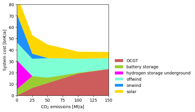

Exercises¶

Explore the model by changing the assumptions and available technologies. Here are a few inspirations, which you do not have to follow in order:

Task 1: Rerun the model with cost assumptions for 2050. You can change the year when loading the technology data.

Task 2: What if either hydrogen or battery storage cannot be expanded? You can remove components with n.remove("StorageUnit", "ComponentName").

Task 3: What if you can either only build solar or only build wind? You can remove components with n.remove ("Generator", "ComponentName").

Task 4: Vary the energy-to-power ratio of the hydrogen storage. What ratio leads to lowest costs? You can change the ratio with n.storage_units.loc["StorageName", "max_hours"] = new_value and adjusting n.storage_units.loc["StorageName", "capital_cost"].

Task 5: On model.energy, you can download capacity factors for onshore wind and solar for any region in the world. Drop offshore wind from the model and use the onshore wind and solar time series from another region of the world. What changes if you select another region? You can read the CSV files from URL with pd.read_csv("URL", index_col=0, parse_dates=True).

Task 6: Add nuclear as another dispatchable low-emission generator (modelled similarly to the OCGT generator). Perform a sensitivity analysis trying to answer how low the capital cost of a nuclear plant would need to be to be chosen in the cost-optimal mix.